
Fairness II: causal
Important note: this week is about whether an insurer may price on gender, directly or through other variables, and about which causal paths from a protected attribute are fair. The algebra below is not contested. Which causal graph describes a real case, which paths are fair, and what the law should require are contested, and my view is one view. A well-argued position I think is wrong can still get full marks.
Summary
Since December 2012 an insurer in the European Union may not use gender to set an individual’s premium. It can still use other risk factors, and some of those depend on gender. The observational criteria compare groups in a table, and the same table can come from different mechanisms. This week writes the mechanism down as a causal model, which makes a new kind of question possible: what would this person’s price have been had the attribute been different?
Counterfactual fairness asks that the answer be the same price. In the simplest example, the red car, any price that depends on the car but not on gender fails this test, and a price that uses both can pass it. Direct and indirect effects split the effect of an attribute along the paths it takes, and the total effect is their sum when the two are defined with matching reference levels. A path-specific criterion removes the effect of the attribute only along the paths judged unfair. On one small model, the counterfactually fair price and the path-specific price differ by the contribution of the path someone judged fair.
Which paths are fair is not something the data can say. One way to judge it, the one this week follows, is by control and responsibility, with moral luck, the control principle and luck egalitarianism. In the red car, a counterfactually fair price that depends on the car needs the attribute that the law forbids an insurer to price an individual on.
Warm-up
The task was to bring one decision in which an attribute is used, or deliberately not used, with one route by which it could affect the outcome, and whether that route is fair. A route is a path in a causal graph: an arrow from the attribute to something, and on to the outcome. Drawing it makes the judgment visible, because the judgment is about particular arrows. “Gender affects the premium” says little; “gender affects how many miles a person drives, and mileage affects claims” names a path someone can defend or object to.
The red car
Pricing without gender
On 1 March 2011 the Court of Justice of the European Union ruled on a question sent to it by the Belgian Constitutional Court, where Test-Achats, a Belgian consumers’ association, had challenged the Belgian law transposing an EU directive that prohibits discrimination based on sex in access to goods and services. The directive prohibited the use of sex as a factor in insurance premiums and benefits, but let member states allow exceptions, provided the actuarial and statistical data behind them were reliable, regularly updated and available to the public. The Court’s press release is headed “Taking the gender of the insured individual into account as a risk factor in insurance contracts constitutes discrimination”, and the Court ruled that the exception was invalid from 21 December 2012.
The European Commission’s guidelines on the ruling say what it covers. From 21 December 2012 the unisex rule applies “without any possible exception in relation to the calculation of individuals’ premiums and benefits in new contracts” (paragraph 5). Gender may still be used “in the calculation of premiums and benefits at the aggregate level, as long as it does not lead to differentiation at individual level”, for example in reserving and internal pricing (paragraph 14). Other risk factors are covered by the rules on indirect discrimination, and “The use of risk factors which might be correlated with gender therefore remains possible, as long as they are true risk factors in their own right” (paragraph 17). Their footnote gives an example from motor insurance: pricing on the size of a car’s engine “should remain possible, even if statistically men drive cars with more powerful engines.”
These notes simplify all this to a model that does not take \(A\) as an input. The observational criteria cannot say whether such a price is fair, because the same table of counts can come from different mechanisms. The mechanism has to be written down.
The red car
ms4ds, section 3.4.1, and Kusner, Loftus, Russell and Silva (2017), the first of whose scenarios this is, describe an insurer that predicts the accident rate (here, claims \(Y\)) of a policy from the color of the car \(X\). An unobserved factor \(U\), aggressive driving, makes a person both more likely to choose a red car and more likely to have an accident. Members of one group, \(A = 1\), are more likely to drive red cars, and no more likely to be aggressive or to have accidents. Kusner et al. take \(A\) to be race; ms4ds takes it to be gender, and so do these notes and the Commission’s guidelines, with \(A = 1\) for a woman.
The graph is \(A \to X \leftarrow U \to Y\). There is no directed path from \(A\) to \(Y\): gender has no effect on claims. The insurer, forbidden to use gender, predicts from the car alone. ms4ds calls this functional independence, \(\hat Y = \hat f(X)\) with \(A\) not an input; Kusner et al. call it fairness through unawareness.
The unaware price
Take a linear version with numbers. Half the drivers are women, so \(A \sim \text{Bernoulli}(1/2)\) and \(\operatorname{Var}(A) = 1/4\); \(U \sim N(0, 1)\), independent of \(A\); car color on a continuous scale, higher for redder, is \(X = 2A + U\); and claims are \(Y = U + \varepsilon\), with \(\varepsilon \sim N(0, 1)\) independent of \((A, U)\).
The least-squares slope of \(Y\) on \(X\) alone is
\[ \frac{\operatorname{Cov}(X, Y)}{\operatorname{Var}(X)} = \frac{\operatorname{Var}(U)}{2^2 \operatorname{Var}(A) + \operatorname{Var}(U)} = \frac{1}{1 + 1} = \frac12 , \]
and since \(E[X] = 1\) and \(E[Y] = 0\), the fitted line is \(\hat Y = \tfrac12 X - \tfrac12\). Women’s average car color is \(2\) and men’s is \(0\), so women’s average predicted claims are \(\tfrac12\) and men’s are \(-\tfrac12\), with claims and prices measured from the average. Average claims are \(0\) in both groups. The price that never looks at gender charges women more, for claims they do not make.
A simulation of 1,000 drivers, and least squares with and without \(A\):
n <- 1000
A <- rbinom(n, 1, 1/2)          # 1 for a woman
U <- rnorm(n)                   # aggression, never observed
X <- 2 * A + U                  # car color
Y <- U + rnorm(n)               # claims
coef(lm(Y ~ X))                 # the price from X alone
(Intercept) X
-0.5454934 0.5115697 coef(lm(Y ~ X + A)) # the price from X and A(Intercept) X A
0.01150287 1.04309699 -2.12880088 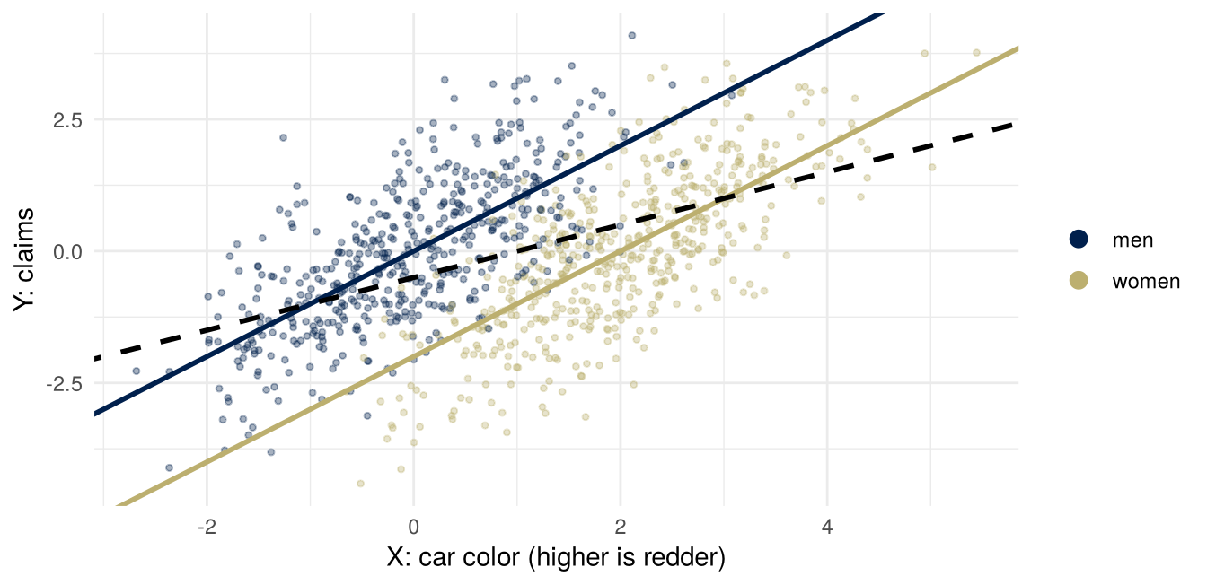
The figure shows the simulated drivers and the population lines. The dashed line is the fit on \(X\) alone. The two solid lines are the best predictions from \(X\) and \(A\), one for each group: at any given color, a woman has lower expected claims than a man.
A counterfactual driver
The reading’s Definition 5 (page 123) gives three steps for a counterfactual in a structural causal model. Abduction: adjust the unobserved variables to be consistent with what was observed. Here \(U = X - 2A = 0.6\). Action: set the attribute, \(A := 0\). Prediction: recompute everything downstream of \(A\) in the modified model, with the abducted \(U\). Her car would have scored \(X = 2 \cdot 0 + 0.6 = 0.6\): two units of her color came from \(A\) rather than from \(U\).
| she, \(A = 1\) | had \(A\) been \(0\) | |
|---|---|---|
| abduction: \(U = X - 2A\) | \(0.6\) | \(0.6\) |
| prediction: \(X = 2A + U\) | \(2.6\) | \(0.6\) |
| price from \(X\) alone, \(\tfrac12 X - \tfrac12\) | \(0.8\) | \(-0.2\) |
| price from \(X\) and \(A\), \(X - 2A\) | \(0.6\) | \(0.6\) |
The unaware price for this driver would have been one unit lower had she been a man. The price that uses \(A\), which is the best prediction from \(X\) and \(A\) in this model, would have been the same.
Counterfactual fairness
Write \(\hat Y(a)\) for the prediction for the same person, with \(U\) abducted from what was observed about them, had \(A\) been set to \(a\). Kusner et al. write \(\hat Y_{A \leftarrow a}(U)\); the reading writes \(\hat Y_{A := a}(E)\), with \(E\) the observed event.
Counterfactual fairness (Kusner et al., Definition 5, page 3). A predictor \(\hat Y\) is counterfactually fair if, for every \(x\) and \(a\), and every value \(a'\) of \(A\),
\[ P\big(\hat Y(a) = y \mid X = x, A = a\big) = P\big(\hat Y(a') = y \mid X = x, A = a\big) \quad \text{for all } y . \]
The distribution is over the values of \(U\) consistent with what was observed; in the red car, \(U\) is determined by \(X\) and \(A\), so it is a single value. Kusner et al. call this “an individual-level definition” (page 3): it compares a person with themselves, not one group with another. The reading calls the same condition counterfactual demographic parity (page 129).
Lemma 1 (Kusner et al., page 5). If \(\hat Y\) is a function of the non-descendants of \(A\) in the causal graph, it is counterfactually fair. A non-descendant of \(A\) takes the same value whatever \(A\) is set to, so any function of non-descendants does too. Kusner et al. add that a predictor can use descendants of \(A\) and still be counterfactually fair, but only where the dependence on \(A\) cancels, which does not happen in general.
The red car, linear. Let \(X = \beta_A A + U\) and \(Y = U + \varepsilon\) with \(\beta_A \neq 0\), \(U\) and \(\varepsilon\) independent of \(A\) and of each other. The least-squares predictor from \(X\) alone is \(\hat Y = \lambda X + \lambda_0\) with \(\lambda = \operatorname{Var}(U) / (\beta_A^2 \operatorname{Var}(A) + \operatorname{Var}(U)) > 0\). For the same \(U\), \(X(a) - X(a') = \beta_A (a - a')\), so \(\hat Y(a) - \hat Y(a') = \lambda \beta_A (a - a') \neq 0\): the unaware predictor is not counterfactually fair. The least-squares predictor from \(X\) and \(A\) is \(E[Y \mid X, A] = X - \beta_A A\), because \(U\) is determined by \((X, A)\); and \(X - \beta_A A = U\), a non-descendant of \(A\), so by Lemma 1 it is counterfactually fair. With \(\beta_A = 2\) these are the two prices in the table. Kusner et al. prove the noise-free case, with \(Y = \gamma U\), as Lemma 3 of their supplement (page 14), and say it in a sentence on page 4: “Regressing Y on X alone obeys the FTU criterion but is not counterfactually fair, so omitting A (FTU) may introduce unfairness into an otherwise fair world.” They add that in this graph “any non-constant estimator that depends only on X is not counterfactually fair” (page 15). A constant price is counterfactually fair without \(A\); a counterfactually fair price that depends on the car at all needs \(A\).
This depends on the model. The fair predictor is built from \(U\), and \(U\) is never observed: it is abducted from \(X\) and \(A\) through the structural equation for \(X\). A different model for \(X\) gives a different \(U\), and a different fair price. Kusner et al. describe three levels of assumption (page 7). Using only the observed non-descendants of \(A\) needs least; using the error terms of an additive model, as here, extracts the most information and assumes the most. Holding \(U\) fixed while gender changes, and recovering it from \(X = 2A + U\), are claims about how the world works, which evidence could support or undermine. Which effects of gender are acceptable is a different kind of claim.
Conditioning or intervening
In this world \(P(Y \mid do(A := 1)) = P(Y \mid do(A := 0))\): there is no directed path from \(A\) to \(Y\). Yet in the fitted \(\hat Y = X - 2A\) the coefficient on \(A\) is \(-2\). The coefficient compares women and men with the same car color. Car color is a collider on the path \(A \to X \leftarrow U\), and among drivers with the same \(X\), a woman’s color owes two units to \(A\), so her \(U\) is two units lower. The coefficient is a statement about conditioning on \(X\); the absence of an effect is a statement about intervening on \(A\).
Direct and indirect effects
A mediation example
The red car has no path from \(A\) to \(Y\) at all. In many cases the attribute does affect the outcome, along some paths that people find acceptable and some that they do not. Keep the insurer and change the world. Annual mileage \(M\), in thousands of miles, depends on gender, and claims \(Y\), in hundreds of pounds a year, depend on mileage and on gender directly:
\[ M = \mu_0 + \alpha A + U_M, \qquad Y = \gamma A + \beta M + U_Y , \]
with \(U_M\) and \(U_Y\) of mean zero, independent of each other and of \(A\), and \(A = 1\) for a woman. The numbers are invented for the arithmetic: \(\mu_0 = 10\), \(\alpha = -4\), \(\beta = 0.25\), \(\gamma = -0.5\). Men drive \(10{,}000\) miles a year on average and women \(6{,}000\); each thousand miles adds £25 a year in expected claims; and at the same mileage, women’s expected claims are £50 a year lower.

Counterfactuals with a mediator
A natural first answer is to compare a woman and a man at the same mileage. Making that precise, and the alternative to it, needs two kinds of counterfactual, both built from \(do(\cdot)\):
- \(Y(a, m)\), the claims under \(do(A := a, M := m)\);
- \(M(a)\), the mileage under \(do(A := a)\).
Combining them, \(Y(a, M(a'))\) is the claims with \(A\) set to \(a\) and mileage set to the value it would have taken under \(A = a'\). When \(a \neq a'\) this is a cross-world quantity: \(Y(1, M(0))\) is a woman driving the miles she would have driven as a man. It is not observable. The reading writes \(Y_{X := 1,\, Z := Z_{X := 0}}\) for the same thing, with \(X\) the treatment and \(Z\) the mediator (page 128); these notes keep \(Z\) for a confounder and \(X\) for covariates.
The controlled direct effect at mileage \(m\) sets the mediator to the same value for everyone: \(\text{CDE}(m) = E[Y(1, m) - Y(0, m)]\). It needs only \(do(\cdot)\).
The decomposition
The total effect is \(\text{TE} = E[Y(1, M(1)) - Y(0, M(0))]\), the same as \(E[Y \mid do(A := 1)] - E[Y \mid do(A := 0)]\). Add and subtract \(E[Y(1, M(0))]\):
\[ \begin{aligned} \text{TE} &= E[Y(1, M(1)) - Y(0, M(0))] \\ &= \underbrace{E[Y(1, M(0)) - Y(0, M(0))]}_{\text{NDE}} \\ &\quad + \underbrace{E[Y(1, M(1)) - Y(1, M(0))]}_{\text{NIE}} . \end{aligned} \]
The natural direct effect changes \(A\) with mileage held at the value it would have taken under \(A = 0\). The natural indirect effect holds \(A\) at \(1\) and changes mileage from \(M(0)\) to \(M(1)\). In words: change gender first, keeping mileage where it would have been; then change mileage, keeping gender at its new value. The second step starts where the first ends, at \(Y(1, M(0))\), so the two add up to the total effect. No model was used, so \(\text{TE} = \text{NDE} + \text{NIE}\) in any model where the expectations exist.
The reading defines the natural indirect effect with \(A\) held at \(0\), \(E[Y(0, M(1)) - Y(0, M(0))]\) (page 128). With that definition the sum of the two natural effects is the total effect only in models where the indirect effect does not depend on the level at which \(A\) is held, such as the linear model below. With an interaction between \(A\) and \(M\) the two can differ.
The natural effects need more than \(do(\cdot)\): they combine two settings of \(A\) for the same person, which no experiment can do. Estimating them from data needs an assumption about the two worlds together. In the model above it is built in, by taking \(U_M\) and \(U_Y\) independent. When the effect is unconfounded, the reading gives the indirect effect as a formula in conditional expectations (page 128).
In the linear model
Put the structural equations into the definitions:
\[ M(a) = \mu_0 + \alpha a + U_M, \qquad Y(a, m) = \gamma a + \beta m + U_Y . \]
Then \(Y(1, m) - Y(0, m) = \gamma\) for every \(m\), so \(\text{CDE}(m) = \gamma\). The NDE holds mileage at \(M(0)\) in both terms, so it is also \(\gamma\). In the NIE, \(Y(1, M(1)) - Y(1, M(0)) = \beta\,(M(1) - M(0)) = \alpha\beta\): the same \(U_M\) appears in \(M(1)\) and \(M(0)\) and cancels. So
\[ \text{CDE}(m) = \text{NDE} = \gamma, \qquad \text{NIE} = \alpha\beta, \qquad \text{TE} = \gamma + \alpha\beta . \]
In a linear model with no interaction, the indirect effect is the product of the coefficients along the path. In the mileage world, \(\text{NDE} = -0.5\), \(\text{NIE} = -4 \times 0.25 = -1\) and \(\text{TE} = -1.5\): women’s expected claims are £150 a year lower than men’s, £100 of it through mileage and £50 directly.
Holding a mediator fixed
\(Y(1, M(0))\) is not an observable outcome; the model supplies it, and every statement about the natural direct effect rests on the model’s assumption about the two worlds together. The tempting substitute is to compare women and men who drive the same number of miles. That holds mileage fixed in the data rather than by intervention, and it can go wrong.
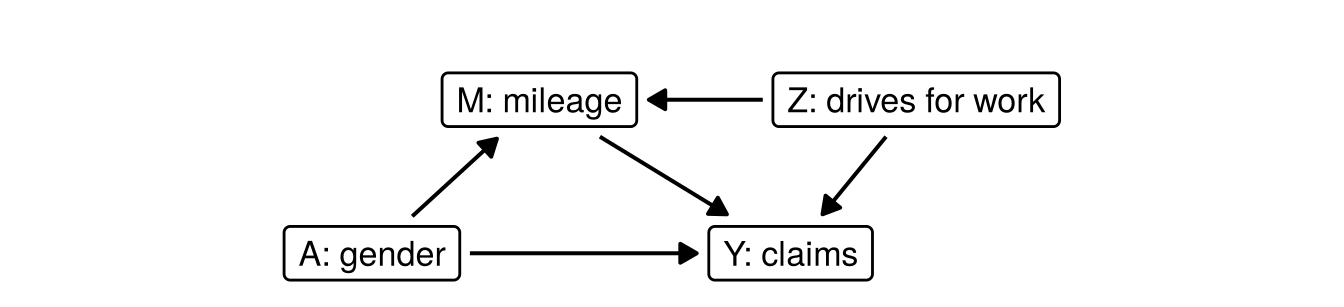
A regression of \(Y\) on \(A\) and \(M\) compares women and men with the same mileage. In the model above, its coefficient on \(A\) is \(\gamma\), the controlled direct effect, because nothing else affects both mileage and claims. Suppose something does: driving for work, \(Z\), adds miles and, beyond what those miles add, adds claims. Then \(M\) is a collider on the path \(A \to M \leftarrow Z \to Y\). Women drive fewer miles on average, so a woman with the same mileage as a man is more likely to drive for work, and at equal mileage her expected claims are higher, relative to his, than the direct effect alone would make them: the coefficient on \(A\) lies above \(\gamma\). Comparing people with the same value of a mediator holds it fixed in the data, which is not the same as holding it fixed by intervention.
Two fair predictors
Before December 2012 the insurer’s best prediction was the full one, \(Y_{\text{full}} = \gamma A + \beta M\), which is \(E[Y \mid A, M]\) in this world. The premiums in this part are population quantities, written without hats: they depend on the unknown parameters \(\mu_0\), \(\alpha\), \(\beta\) and \(\gamma\), which an insurer would estimate.
The first is the counterfactually fair premium and the second the path-specific one. On this model both can be computed by hand.
The comparison
| premium | formula | gap, women minus men |
|---|---|---|
| full | \(\gamma A + \beta M\) | \(\gamma + \alpha\beta\), the TE |
| path-specific | \(\beta M\) | \(\alpha\beta\), the NIE |
| counterfactually fair | \(\beta(M - \alpha A)\) | \(0\) |
The three differ, for every driver, by
\[ Y_{\text{full}} - Y_{\text{PS}} = \gamma A, \qquad Y_{\text{PS}} - Y_{\text{CF}} = \alpha\beta A . \]
The first difference is the contribution of the direct path, and the second is the contribution of the path through mileage. The two fair premiums differ by the contribution of the path someone judged fair. Neither criterion says which path that is.
The level
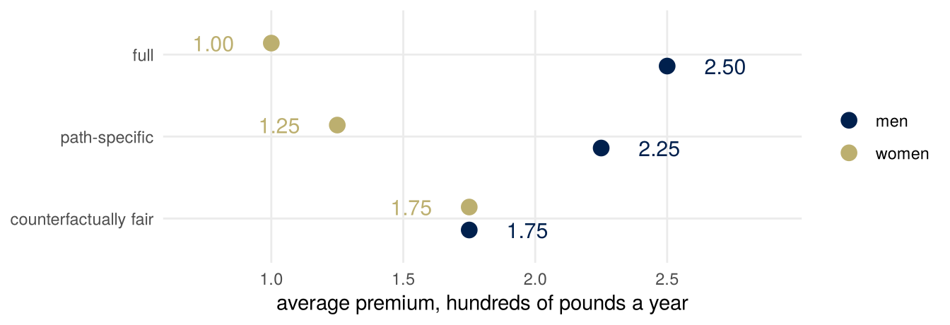
As constructed, the three premiums collect different amounts: in the mileage world, with as many women as men, £175, £200 and £250 a policy on average, while the average claim is £175. Men pay £250 under all three, so the full premium is the cheapest or equal for every driver, and choosing between them involves no trade-off. Adding a constant to a premium changes neither its gaps nor its fairness properties: the path-specific premium still takes no \(A\), and the counterfactually fair one is still a function of \(U_M\). Shifting each so that it collects the average claim gives:
| premium, each collecting £175 a policy | men | women |
|---|---|---|
| full | £250 | £100 |
| path-specific, less £25 | £225 | £125 |
| counterfactually fair, less £75 | £175 | £175 |
Now the choice moves money between groups: men pay least under the counterfactually fair premium and women under the full one, and the insurer collects the same either way.
The level is a choice the definitions do not make. Pricing everyone as the full model would price them had they been women, \(\gamma + \beta(\mu_0 + \alpha + U_M)\), is counterfactually fair too, and differs from the premium above by a constant. The two groups’ average counterfactually fair premiums are equal here because \(U_M\) is independent of \(A\) in this model. In a model where a non-descendant of \(A\) is associated with \(A\), a counterfactually fair premium can differ between groups.
Two graphs, the same data
The premiums above were computed from the model as written. An insurer has records of gender, mileage and claims, and has to choose a graph before it can compute anything. Suppose the world is the one in “Holding a mediator fixed” above. \(Z\) is now a score for how much a person drives for work, normally distributed with mean \(1/4\) and variance \(3/16\) and independent of gender. Each unit of \(Z\) adds \(4{,}000\) miles a year and, beyond what those miles add, £100 of claims; the insurer does not record it:
\[ M = 9 + 4Z - 4A + U_M, \qquad Y = -0.5A + 0.25M + Z + U_Y , \]
with \(U_M\) and \(U_Y\) normal, \(\operatorname{Var}(U_M) = 4\), and half the drivers women. Men still drive \(10{,}000\) miles on average. The direct effect is \(\gamma = -0.5\) and the effect through mileage \(\alpha\beta = -1\), as before.
An analyst who draws the lecture’s graph, without \(Z\), fits it by regressing claims on gender and mileage. The coefficients are the world’s plus the effect of \(Z\), which is 1, times the coefficients of a regression of \(Z\) on \(A\) and \(M\), which are \(3/7\) and \(3/28\) (\(\operatorname{Var}(M) = 11\), \(\operatorname{Cov}(A, M) = -1\), \(\operatorname{Cov}(Z, M) = 0.75\)):
| direct | through mileage | total | |
|---|---|---|---|
| graph without \(Z\), fitted | \(-0.07\) | \(-1.43\) | \(-1.5\) |
| graph with \(Z\) (the world) | \(-0.5\) | \(-1.0\) | \(-1.5\) |
In the world, mileage and claims are jointly normal for women and for men, with the same variances and covariance in both groups. The graph without \(Z\) has an arrow between every pair of the three variables it records, so it fits such records exactly: the records alone cannot tell the two graphs apart. (Had \(Z\) been yes or no, a quarter of drivers driving for work, the means, variances and covariances would be the same, but the average claim given gender and mileage would curve slightly in mileage, with a slightly different slope for women and men, which the linear graph without \(Z\) would miss.)
The path-specific premium differs between the graphs. Fitted without \(Z\), it is \(0.357\,M\) plus a constant, and women pay £143 less than men on average; in the world, it is \(0.25\,M + Z\) plus a constant, which cannot be charged without recording \(Z\), and the gap is £100. Take the counterfactually fair premium to be the least-squares premium on \(M - \alpha A\), the mileage a driver would have had as a man; fairness alone does not pick a unique premium. It does not differ between the graphs: \(Z\) is independent of gender, so both graphs agree that \(M - \alpha A\) is a non-descendant of \(A\) and both have \(\alpha = -4\), and the slope is \(0.357\) under either. A criterion that removes every path from \(A\) needs less of the graph than one that keeps some, but it removes the path through mileage too. With the structure uncertain and a premium to set, choosing between the two is a decision about which error to risk.
Whose judgment
The criteria need a list of fair and unfair paths, and the sources are explicit that the list comes from outside the data.
Kusner et al.’s supplementary material (page 15) adapts the Berkeley admissions example, with \(A\) an indicator of a female applicant and \(X\) the course applied to: “Our judgment is that the higher rejection among female than male applicants is acceptable, if the mechanism A → X is interpreted as a choice which is under the control of the applicant.”
The reading, Barocas, Hardt and Narayanan, says of the same example that treating department choice as the applicant’s own inherent preference “is a substantive judgment that may not be a fact” (page 119). It describes worlds consistent with the same data in which discrimination runs through department choice: a program advertised in a way that discouraged women from applying, or a department known for hostility to women, and concludes: “Accepting the indirect path as non-discriminatory is to assert that all these scenarios we described are deemed implausible.”
Nabi and Shpitser: “The specific paths which correspond to discrimination are a domain specific issue.” Their example is a physical fitness test, which may be appropriate for a job in construction and not for one in accounting, so that the same path from gender through the test to hiring may or may not be discriminatory (arXiv version, page 4).
ms4ds draws a related distinction between a shallow counterfactual and a deep one (section 3.4.1.1). A shallow counterfactual changes the name on an application and keeps everything else in the person’s life the same; a deep one asks how the application would differ had the person had that name all their life. The counterfactually fair premium is a deep counterfactual along every path; the path-specific premium is deep along some paths and shallow along the others.
Dropping the attribute and refitting
An insurer that may not use \(A\) can refit claims on mileage alone. The least-squares slope is \(\operatorname{Cov}(Y, M) / \operatorname{Var}(M)\), and \(\operatorname{Cov}(Y, M) = \gamma \operatorname{Cov}(A, M) + \beta \operatorname{Var}(M)\), so
\[ \text{slope} = \beta + \gamma\,\frac{\operatorname{Cov}(A, M)}{\operatorname{Var}(M)} , \]
with \(\operatorname{Cov}(A, M) = \alpha \operatorname{Var}(A)\) and \(\operatorname{Var}(M) = \alpha^2 \operatorname{Var}(A) + \operatorname{Var}(U_M)\).
The refitted premium’s gap between women and men is the slope times \(E[M \mid A = 1] - E[M \mid A = 0] = \alpha\):
\[ \alpha\beta + \gamma\,\frac{\alpha^2 \operatorname{Var}(A)}{\operatorname{Var}(M)} = \text{NIE} + R^2\,\text{NDE} , \]
where \(R^2 = \alpha^2 \operatorname{Var}(A)/\operatorname{Var}(M)\) is the share of the variance of mileage explained by gender. With \(\operatorname{Var}(A) = 1/4\) and \(\operatorname{Var}(U_M) = 4\), \(\operatorname{Var}(M) = 8\), \(\operatorname{Cov}(A, M) = -1\), the slope is \(0.25 + (-0.5)(-1)/8 = 0.3125\) and the gap is \(-1.25\): the path through mileage, \(-1\), and half of the direct effect, \(-0.25\), which returns because mileage stands in for gender. The refitted premium does not take \(A\) as an input, and its slope on mileage, \(0.3125\), is above \(\beta = 0.25\).
Nabi and Shpitser’s method fits the model closest to the data, by likelihood, among those in which the path-specific effect judged unfair is held within bounds. When the outcome model is linear and the unfair effect is the natural direct effect, they note that holding it at zero “coincides to simply dropping A from the outcome regression” (arXiv version, page 6). In the mileage world that fitted outcome regression has slope \(0.3125\) on mileage, and the fitted model has no direct effect by construction. To predict for a new case they average the mediator out, using \(\tilde E[Y \mid A, C] = \sum_M \tilde E[Y \mid A, M, C]\, \tilde p(M \mid A, C)\) (page 5), so their prediction depends on \(A\) through the mileage the fitted model expects; its gap between women and men is again \(-1.25\). Measured against the world the data came from, that gap includes half of the direct effect. The path-specific premium \(\beta M\) uses the world’s slope, \(0.25\), which a regression that leaves \(A\) out does not estimate. Which of the two is the fair price of a mile depends on whether the fitted model or the world is what the criterion is about.
With an interaction
The decomposition of the total effect is an identity, and with an interaction the natural effects in it depend on their reference levels. Let
\[ M = \mu_0 + \alpha A + U_M, \qquad Y = \gamma A + \beta M + \delta A M + U_Y , \]
and write \(\text{NDE}_a\) for the natural direct effect with mileage held at \(M(a)\), and \(\text{NIE}_a\) for the natural indirect effect with \(A\) held at \(a\). Since \(E[M(0)] = \mu_0\) and \(E[M(1)] = \mu_0 + \alpha\):
\[ \begin{aligned} \text{TE} &= \gamma + \alpha\beta + \delta(\mu_0 + \alpha) \\ \text{NDE}_0 &= E[Y(1, M(0)) - Y(0, M(0))] = \gamma + \delta\mu_0 \\ \text{NIE}_1 &= E[Y(1, M(1)) - Y(1, M(0))] = \alpha(\beta + \delta) \\ \text{NDE}_1 &= E[Y(1, M(1)) - Y(0, M(1))] = \gamma + \delta(\mu_0 + \alpha) \\ \text{NIE}_0 &= E[Y(0, M(1)) - Y(0, M(0))] = \alpha\beta . \end{aligned} \]
Both \(\text{NDE}_0 + \text{NIE}_1\) and \(\text{NDE}_1 + \text{NIE}_0\) equal the total effect: the decomposition holds with the reference levels paired this way, and not in general. The pair the reading defines, \(\text{NDE}_0\) and \(\text{NIE}_0\), sums to \(\text{TE} - \alpha\delta\). The product of coefficients \(\alpha\beta\) is \(\text{NIE}_0\), which is not the indirect effect that pairs with \(\text{NDE}_0\). With \(\delta = 0\) both pairings give \(\gamma\) and \(\alpha\beta\).
Luck and responsibility
Moral luck
Dana Nelkin’s encyclopedia entry opens: “Moral luck occurs when an agent can be correctly treated as an object of moral judgment despite the fact that a significant aspect of what she is assessed for depends on factors beyond her control.”
ms4ds, section 3.4.2: “Moral luck refers to how our evaluation of whether someone has done good or not can depend on factors which are outside of that person’s control. The control principle says that we should only judge people to the extent that the factors we judge them on are under their control.” The same section gives the control principle as one justification for treating attributes such as race or gender as sensitive in the first place: they are commonly understood to be outside a person’s control.
The middle view of equality of opportunity, in chapter 4 of Barocas, Hardt and Narayanan’s book, holds that decision makers “must, to some degree, treat seemingly dissimilar people similarly when the causes of these dissimilarities are themselves problematic” (page 84). For employment, the book suggests that hiring managers might assess people by the opportunities they have had, “discounting certain differences in qualifications that might owe to factors outside their control” (page 85). It names insurance as a case: “The middle view has particular purchase in the case of insurance, where we really might want insurers to ignore the additional costs that they are likely to face in setting the price of a policy for someone with an expensive pre-existing condition outside the person’s control” (chapter 4, page 85).
Luck egalitarianism
Luck egalitarianism is a related view about who gets what. Kasper Lippert-Rasmussen’s encyclopedia entry opens with the observation that some people end up worse off than others partly because of bad luck, and its section 7 sets out the distinction between brute luck, risks a person did not choose to take, and option luck, how a gamble the person chose turns out: “Luck-egalitarians, for example, often separate option luck and brute luck and deny that instances of differential option luck are unjust.” On that view, two people who take the same gamble and end up unequal because one of them lost have no claim of justice against the result; an inequality that comes from brute luck, such as an illness nobody chose, can be unjust. The entry also records that views on option luck differ: whether justice requires its effects to stand, permits correcting them, or requires correcting some of them.
Moral luck names a problem: how we judge what people did can depend on things they did not control. The control principle is one response to it. Luck egalitarianism is about how goods and burdens should be distributed, and its distinction between brute and option luck is a related response there. This course takes them together because they ask the same question, what a person is responsible for. A premium is a burden distributed among policyholders.
Barocas, Hardt and Narayanan’s chapter 4 marks the limit of the formal tools here: “many of the concepts in this chapter, such as whether a decision subject has control over an attribute used for decision making, cannot be expressed in the statistical language of conditional probabilities and expectations” (chapter 4, page 92). A causal graph does not settle it either. It can show that a path exists. On the control principle, whether the person controls what happens along it decides whether the path is fair.
A mediator shaped by the attribute
Mileage is a rating factor with an obvious connection to risk: more miles, more exposure. In the mileage world it also differs by gender, and part of what makes women’s claims lower runs through it. Whether the path \(A \to M \to Y\) is fair depends on why mileage differs. If the difference reflects choices people control, the control principle counts the path as fair. If it reflects who does which job, or which share of caring, it is less clear that the choice was the person’s. The Berkeley example has the same shape, with department choice in the place of mileage, and the reading’s alternative worlds are the argument that a mediator’s appearing to be a choice does not make it one. The Commission’s guidelines answer the legal version of the question: a factor correlated with gender may be used “as long as” it is a true risk factor “in their own right” (paragraph 17).
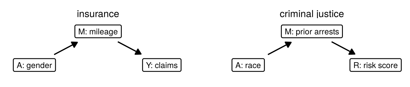
A second mediator makes the question sharper. A risk score used in criminal justice may take prior arrests as an input, and race can affect prior arrests: arrests record where police look as well as what people do, and they can follow from less economic opportunity. Here the mediator itself can record unequal treatment, and a path through it is harder to call fair than a path through mileage.
A framework and a criterion
ms4ds, after showing what the unaware model does in the red car world: “But there may be a deontological argument in favor of functional independence, including empirical evidence that people generally believe a process with functional independence is more fair” (section 3.4.1). A deontologist may hold that a decision should not take a protected attribute as an input, whatever the consequences. In the red car world that rule produces a price that is not counterfactually fair, unless it ignores the car too, and a counterfactually fair price that depends on the car breaks it. Since December 2012, EU law forbids the second for an individual’s premium. Whether a framework implies a criterion, and whether the two can disagree like this, is a question for the class.
Intersectionality
With two attributes, \(A_1\) and \(A_2\), a model with an interaction,
\[ Y = \gamma_1 A_1 + \gamma_2 A_2 + \delta A_1 A_2 + \dots , \]
gives the effect of \(A_1\) as \(\gamma_1\) when \(A_2 = 0\) and \(\gamma_1 + \delta\) when \(A_2 = 1\). A model without the interaction, \(\delta = 0\), assumes that the effect of one attribute is the same at every level of the other: that being a woman has the same effect whatever one’s race, for example. Yang, Loftus and Stoyanovich build causal models for intersectional fairness in which, in their words, “we generally assume that f_j contains non-additive interactions between sensitive attributes” (arXiv version, page 3), and keep main effects and second-order interactions in their examples. In such a model, each effect of one attribute is stated at a level of the other.
Permissions with a time stamp
A fairness criterion that conditions on a variable \(V\), or allows \(A\)’s influence along paths through \(V\), works as a permission: it accepts whatever group disparity \(V\) already has. Every variable is determined at some point in a person’s life, so a criterion can be placed on a timeline by the latest variable it allows. On a hiring timeline, the attribute \(A\), then qualifications \(X\), then job performance \(Y\), then the decision \(D\), demographic parity and counterfactual fairness allow nothing after \(A\). Path-specific fairness and conditional statistical parity allow chosen mediators such as \(X\). Equality of opportunity conditions on the outcome \(Y\) itself, and so, under this reading, essentially justifies all disparities. A criterion that allows later variables lets more accumulated history count as justified.
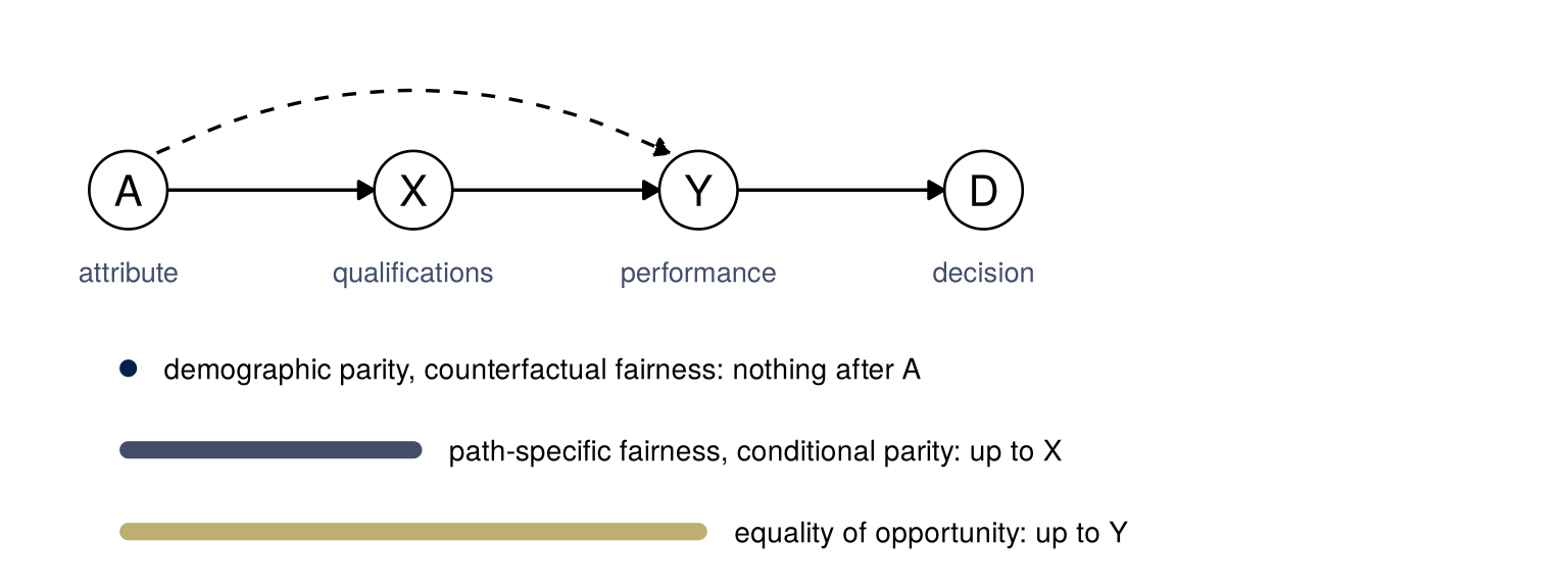
The dashed arrow is a direct effect of \(A\) at a later stage. Whether the disparity a later variable has should count as justified depends on how it got there.
Which arrows should count?
Causal structure says what a criterion permits; whether it should permit it depends on the moral character of each path from \(A\). Three types, as a diagnostic rather than a settled theory:
- Injustice-transmitting: the effect reflects discrimination or structural disadvantage, such as unequal schooling. Blocking it reduces unfairness.
- Justified mediation: the effect runs through a neutral mechanism, such as a person’s own choices or a legitimate signal. Allowing it is fine.
- Injustice-responsive: the effect records harm or need that the decision should respond to, as in allocating care by health need (Obermeyer et al., 2019). Blocking it is itself a harm.
The moral luck of the lecture gives a way to read each mediator: how much control did the person have over it? Choices are closest to what the control principle allows us to judge, and are the natural home of justified mediation. A neighborhood, a school’s quality or how heavily an area is policed are circumstantial luck, luck “in the circumstances in which one finds oneself” in Nelkin’s entry, and often transmit injustice. Traits and dispositions shaped before any choice are constitutive luck, luck in who one is. A criterion that allows later variables allows more choice-like mediators, and also everything luck did to the earlier ones: qualifications at a given time already contain the circumstances before it.
Control is not the same as justice. Something outside a person’s control is not automatically an injustice, and something a person chose may have been shaped by unjust circumstances; this is the worry that constitutive luck undermines the control principle. One variable can carry both kinds of effect, and data on the variable alone do not separate them.
The same causal graph can call for opposite criteria, depending on how each arrow is read.
Lenses
The six lenses, by name:
- Goal selection. What are we optimizing or predicting?
- Data selection. Who is in the data?
- Honest reporting. Which comparison gets reported?
- Justice. Who bears the error?
- Ownership. You have to choose, so choose, and defend it.
- Leverage. What can be changed, and how?
Each ends with the same two words: and why? Three of them apply to this week’s material.
Data selection. Who is in the data? Each driver is in the data once, with one value of the attribute. The same driver with the other value, and \(Y(1, M(0))\), are not observable: the model fills them in by abduction. A counterfactual criterion is a statement about people the insurer has never observed, and it is only as good as the model that supplies them.
Ownership. You have to choose, so choose, and defend it. Which paths are fair; the level of each premium, and so which group pays toward the other’s claims; whether to price without the attribute, as the law requires, or with it, as any counterfactually fair price that depends on the car does in the red car world. Given a choice, the criteria give its consequences.
Leverage. What can be changed, and how? What things are considered “controlled for” or “held fixed,” and is that realistic? Abduction holds \(U\) fixed for the counterfactual driver, which assumes the model’s \(U\) is a property of the person that would not change with the attribute. The natural direct effect holds mileage at \(M(0)\), which for a woman is a mileage she is never observed at. Equal mileage in a regression is mileage held fixed in the data, not by intervention, and the two differ when something else drives both mileage and claims.
And why? An insurer prices on the variables it is allowed to use, and the path-specific premium in the mileage world takes no gender as an input. A price that never mentions the attribute can still include an indirect effect that someone judged fair. Who judged it, and on what grounds?
Readings
Required
- Barocas, Hardt and Narayanan, Fairness and Machine Learning: Limitations and Opportunities (MIT Press, 2023), chapter 5, Causality: “Graphical discrimination analysis” through the end of “Counterfactual discrimination analysis”, pages 117 to 131 (printed page numbers; a PDF viewer shows them as 127 to 141). Direct effects, indirect paths, counterfactuals and Definition 5, quantitative path analysis, counterfactual discrimination criteria and counterfactuals in the law. The chapter writes \(X\) for the treatment and \(Z\) for the mediator.
- Re-read Loftus, Modern Statistics 4 Data Science, section 3.4, Causality and ethics: the red car, counterfactual fairness, shallow and deep counterfactuals, moral luck and path-specific counterfactual fairness.
Optional
- The same book, chapter 5, “Validity of causal modeling” (pages 132 to 137): whether categories such as race and gender can be variables in a causal model at all.
- The same book, chapter 4, “Tensions between the different views” through “The cost of fairness” (pages 85 to 92).
- Lippert-Rasmussen, Justice and Bad Luck, The Stanford Encyclopedia of Philosophy, first published 20 June 2005, substantive revision 2 February 2023: the introduction and section 7, option luck and brute luck.
- Kusner, Loftus, Russell and Silva, Counterfactual Fairness, Advances in Neural Information Processing Systems 30 (NIPS 2017), https://proceedings.neurips.cc/paper_files/paper/2017/file/a486cd07e4ac3d270571622f4f316ec5-Paper.pdf: sections 1 to 4. The proceedings record gives no page range; page numbers in these notes are those of the arXiv version, 1703.06856v3, which also has the supplement.
- Chiappa, Path-Specific Counterfactual Fairness, Proceedings of the AAAI Conference on Artificial Intelligence 33(01), 2019, 7801–7808: the introduction.
- Nabi and Shpitser, Fair Inference on Outcomes, Proceedings of the AAAI Conference on Artificial Intelligence 32(1), 2018, https://doi.org/10.1609/aaai.v32i1.11553. The DOI record gives no page range; page numbers in these notes are those of the arXiv version, 1705.10378v4.
- Yang, Loftus and Stoyanovich, Causal Intersectionality and Fair Ranking, 2nd Symposium on Foundations of Responsible Computing (FORC 2021), LIPIcs 192, 2021, 7:1–7:20, https://doi.org/10.4230/LIPIcs.FORC.2021.7. Page numbers in these notes are those of the arXiv version, 2006.08688v1.
Cited in the text and not assigned
Court of Justice of the European Union, Press Release No 12/11, “Taking the gender of the insured individual into account as a risk factor in insurance contracts constitutes discrimination”, Luxembourg, 1 March 2011, on the judgment in Case C-236/09, Association belge des Consommateurs Test-Achats ASBL and Others v Conseil des ministres, https://curia.europa.eu/site/upload/docs/application/pdf/2011-03/cp110012en.pdf. I have read the press release, not the judgment.
European Commission, “Guidelines on the application of Council Directive 2004/113/EC to insurance, in the light of the judgment of the Court of Justice of the European Union in Case C-236/09 (Test-Achats)”, 2012/C 11/01, Official Journal of the European Union C 11, 13 January 2012, 1–11, https://eur-lex.europa.eu/legal-content/EN/TXT/PDF/?uri=OJ:C:2012:011:FULL: paragraphs 5, 14 and 17 and footnote 3 to paragraph 17.
Loftus, Joshua R., “It’s About Time: Fairness and Temporal Depth”, NeurIPS 2023 Workshop on Algorithmic Fairness through the Lens of Time, https://neurips.cc/virtual/2023/78068.
Obermeyer, Ziad, Brian Powers, Christine Vogeli and Sendhil Mullainathan, “Dissecting racial bias in an algorithm used to manage the health of populations”, Science 366(6464), 2019, 447–453, https://doi.org/10.1126/science.aax2342.
Nelkin, Dana K., “Moral Luck”, The Stanford Encyclopedia of Philosophy, first published 26 January 2004, substantive revision 20 January 2025, https://plato.stanford.edu/entries/moral-luck/: the opening sentence; section 1, on circumstantial and constitutive luck.