Fairness I: observational

Joshua Loftus

Week 7

Part 1: Scores that sort people

Part 2: Differing definitions of fairness

Part 3: Conflicting definitions

Part 4: Remedies and their costs

Part 5: Where disparities come from

What you brought

For the rule you brought: who pays when it wrongly says yes? Who pays when it wrongly says no? Are they the same people?

Part 1: Scores that sort people

Who sees a job ad

An advertiser chooses who may see an ad. The platform then chooses who does see it, by predicting who is likely to click.

Ali and colleagues ran job ads on Facebook aimed at the same audience. Ads for jobs in the lumber industry reached an audience 72% white and 90% male; ads for supermarket cashiers, 85% female; ads for taxi companies, 75% Black. Figure 8 of arXiv:1904.02095 (page 12).

In 2022 Meta settled a US Justice Department case over housing ads. It built a system to bring the audience that sees a housing ad closer to the eligible audience, by sex and by estimated race or ethnicity.

Ali, Sapiezynski, Bogen, Korolova, Mislove and Rieke (2019), “Discrimination through Optimization: How Facebook’s Ad Delivery Can Lead to Biased Outcomes,” Proceedings of the ACM on Human-Computer Interaction 3(CSCW), 1–30, doi:10.1145/3359301, pages 2 and 12 of arXiv:1904.02095v5. US Department of Justice, United States v. Meta Platforms, Inc. (S.D.N.Y.), case page, https://www.justice.gov/crt/case/united-states-v-meta-platforms-inc-fka-facebook-inc-sdny, and US Attorney’s Office, S.D.N.Y., press release of 9 January 2023.

Fraud checks on universal credit advances

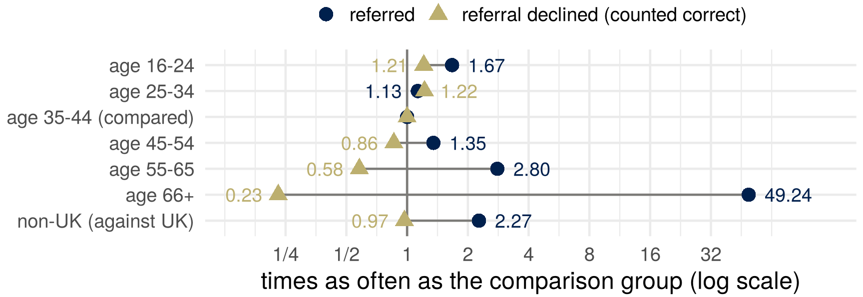
The DWP scores each request for an advance; high-risk ones go to a caseworker, who is not told the model sent them. Its 2025 fairness assessment compares groups on two numbers, and judged the model “reasonable and proportionate to continue operating”:

Department for Work and Pensions (2025), “UC Advances Model: Fairness Assessment,” 17 July 2025, https://www.gov.uk/government/publications/fairness-assessment-including-statistical-analysis-of-the-universal-credit-advances-machine-learning-model-1-april-2024-to-31-march-2025: paragraphs 10, 15, 26; annex Tables 1 to 4. Ages 66+ are 0.1% of requests.

Pretrial risk scores in Broward County

COMPAS: a risk score from 137 questions, none of them about race, sold by Northpointe; a decile from 1 to 10. Broward County, Florida, used it in pretrial decisions. ProPublica (May 2016): the scores of more than 7,000 people assessed in 2013 and 2014, and whether each was arrested again within two years. In the article: Two Shoplifting Arrests.

Convention: \(Y = 1\) is a new arrest within two years; \(\hat Y = 1\) is decile 5 or above, the county’s “medium” and “high”; \(A\) is race as recorded, Black or white.

\(1\) is the bad outcome. Flagged and selected mean the same: \(\hat Y = 1\), picked out by the score, for detention, a fraud check or an ad. The book’s examples run the other way.

Angwin, Larson, Mattu and Kirchner (2016), “Machine Bias,” ProPublica, 23 May 2016, https://www.propublica.org/article/machine-bias-risk-assessments-in-criminal-sentencing; Larson, Mattu, Kirchner and Angwin (2016), “How We Analyzed the COMPAS Recidivism Algorithm,” ProPublica, 23 May 2016, https://www.propublica.org/article/how-we-analyzed-the-compas-recidivism-algorithm.

ProPublica’s table

		flagged	not flagged	across the row
Black defendants	re-arrested	1,369	532	FNR 28%
	not re-arrested	805	990	FPR 45%
white defendants	re-arrested	505	461	FNR 48%
	not re-arrested	349	1,139	FPR 23%

Across a row, conditioning on the truth: \(\text{TPR} = P(\hat Y = 1 \mid Y = 1)\), \(\;\text{FNR} = 1 - \text{TPR}\), \(\;\text{FPR} = P(\hat Y = 1 \mid Y = 0)\).

Of those not re-arrested, 805 of 1,795 Black defendants had been flagged, against 349 of 1,488 white defendants.

A test rejects a true null with probability \(\alpha\) and misses a false one with probability \(\beta\). Which rates are these, with what as the null?

Counts: ProPublica’s compas-scores-two-years.csv (github.com/propublica/compas-analysis), 6,150 people recorded as African-American or Caucasian. Rates: Barocas, Hardt and Narayanan (2023), Tables 3.1 and 3.2, page 47.

The vendor’s reply

	re-arrested, of those flagged	not re-arrested, of those not flagged
Black defendants	1,369 of 2,174: PPV 63%	990 of 1,522: NPV 65%
white defendants	505 of 854: PPV 59%	1,139 of 1,600: NPV 71%

Down a column, conditioning on the flag: \(\text{PPV} = P(Y = 1 \mid \hat Y = 1)\), \(\;\text{NPV} = P(Y = 0 \mid \hat Y = 0)\).

The replies: of those flagged, about the same share was re-arrested in both groups, and the same decile meant about the same re-arrest rate. ProPublica sorted people by what happened; the replies sorted them by what the score said.

The replies as summarized in Chouldechova (2017), “Fair Prediction with Disparate Impact: A Study of Bias in Recidivism Prediction Instruments,” Big Data 5(2), 153–163, doi:10.1089/big.2016.0047, section 1.

Which number should be equal?

If the score has to treat Black and white defendants the same in one respect, which number would you want to be equal:

• as a defendant who will not reoffend;
• as the judge reading the flag;
• as a member of the public?

Then the fraud checks: a claimant who is not committing fraud, the caseworker, a taxpayer. One sentence each. Say why.

Part 2: Differing definitions of fairness

Independence, separation, sufficiency

	the score \(R\)	the flag \(\hat Y\)	on the COMPAS table
independence (demographic parity)	\(R \perp A\)	equal share selected	fails: 59% against 35%
separation (error rate parity)	\(R \perp A \mid Y\)	equal FPR and equal FNR	fails at every cutoff from 2 to 10
sufficiency	\(Y \perp A \mid R\)	equal PPV and equal NPV	nearer: PPV 63% and 59%, NPV 65% and 71%

Predictive parity is equal PPV alone, a relaxation of sufficiency. Each criterion is a property of the joint distribution of \((A, R, Y)\).

Barocas, Hardt and Narayanan (2023), Fairness and Machine Learning: Limitations and Opportunities, MIT Press, https://fairmlbook.org, chapter 3, “Statistical non-discrimination criteria” through “Sufficiency,” pages 54 to 61.

Calibration by group

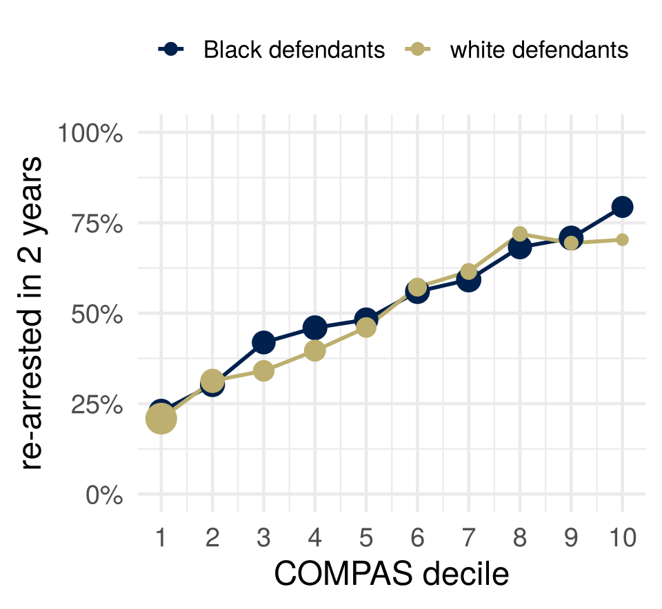
Calibrated by group: \(P(Y = 1 \mid R = r, A = a) = r\) for every \(r\) and \(a\). Deciles are not probabilities: the figure checks that a decile means about the same rate in both groups. Calibration by group implies sufficiency.

A cutoff need not keep it. The PPV is the average re-arrest rate over the deciles selected: 47% of the Black defendants selected are in deciles 8 to 10, against 32% of the white, so the PPVs differ.

Barocas, Hardt and Narayanan (2023), chapter 3, “Calibration and sufficiency,” pages 61 to 63, and page 71.

Two calibrated scores

A score that gives everyone the population’s base rate is calibrated.

A score that is perfect in one group and gives the other group its base rate is calibrated by group.

Calibration checks that the score means what it says. It does not say the score is any good, or that it treats the groups alike.

Barocas, Hardt and Narayanan (2023), chapter 4, “Calibration,” pages 93 and 94.

Part 3: Conflicting definitions

Can all four be equal?

Two groups. In one, 51% are re-arrested; in the other, 39%.

Can one score have the same FPR, the same FNR, the same PPV and the same NPV in both groups: separation and sufficiency at once?

PPV from the rates

One group, prevalence \(p = P(Y = 1)\), a flag \(\hat Y\) with rates FPR and FNR.

\[ P(\hat Y = 1) \;=\; p\,(1 - \text{FNR}) + (1 - p)\,\text{FPR} \]

\[ \text{PPV} \;=\; P(Y = 1 \mid \hat Y = 1) \;=\; \frac{p\,(1 - \text{FNR})}{p\,(1 - \text{FNR}) + (1 - p)\,\text{FPR}} \]

The numerator is the true positives, the denominator everyone flagged.

The significance filter: a share \(p\) of the hypotheses tested are true, tests have level \(\alpha\) and power \(1 - \beta\). The probability that a rejection is a true discovery is this formula with \(\alpha\) for FPR and \(\beta\) for FNR.

Chouldechova’s identity

\[ \frac{1 - \text{PPV}}{\text{PPV}} \;=\; \frac{(1 - p)\,\text{FPR}}{p\,(1 - \text{FNR})} \]

\[ \text{FPR} \;=\; \frac{p}{1 - p}\cdot\frac{1 - \text{PPV}}{\text{PPV}}\cdot(1 - \text{FNR}) \]

Four quantities, one equation. Fix any three and the fourth is determined.

Chouldechova (2017), “Fair Prediction with Disparate Impact: A Study of Bias in Recidivism Prediction Instruments,” Big Data 5(2), 153–163, doi:10.1089/big.2016.0047, equation (2.6), section 2.3.

COMPAS in the identity

When two groups differ in prevalence \(p\), a flag with the same positive predictive value in both, strictly between \(0\) and \(1\), has a different false positive rate or a different false negative rate in the two groups.

With equal PPV and equal FNR, dividing the identity for one group by the other gives \(\text{FPR}_a / \text{FPR}_b\) as the odds ratio, 1.63. The observed ratio is 1.91 \(=\) 1.63 \(\times\) 0.85 \(\times\) 1.38: the odds ratio, the ratio of \((1 - \text{PPV})/\text{PPV}\), and the ratio of TPRs.

Impossibility for a flag

When base rates differ (\(Y \not\perp A\)), a flag that is informative (\(\hat Y \not\perp Y\)) and has \(0 < \text{FPR} < 1\) in each group satisfies at most one of the three criteria.

• Independence and sufficiency: only if \(Y \perp A\).
• Independence and separation: only if \(Y \perp A\) or \(\hat Y \perp Y\).
• Separation and sufficiency: only if \(Y \perp A\), when \(0 < \text{FPR} < 1\).

For COMPAS the base rates differ, so choosing one criterion gives up the other two.

Barocas, Hardt and Narayanan (2023), chapter 3, Propositions 2, 3 and 5, pages 65 to 67.

Impossibility for a score

• calibration within groups, condition A: in each group, people scored \(v\) are positives with frequency \(v\);
• balance for the negative class, B: the negatives’ average score is the same in both groups;
• balance for the positive class, C: likewise for the positives.

Theorem 1.1: all three hold only if prediction is perfect (the features determine the outcome) or the base rates are equal.

In the authors’ reading, ProPublica pointed at B and C failing, the replies at A holding. Even these weaker versions of equal error rates conflict with calibration.

Kleinberg, Mullainathan and Raghavan (2017), “Inherent Trade-Offs in the Fair Determination of Risk Scores,” 8th Innovations in Theoretical Computer Science Conference (ITCS 2017), LIPIcs 67, 43:1–43:23, doi:10.4230/LIPIcs.ITCS.2017.43, section 1; theorem numbering of arXiv:1609.05807v2, the version linked from the readings.

Which would you give up?

Equal predictive value or equal error rates: the two cannot both hold. Which would you require, and which would you give up? Who do you owe the explanation to?

Who pays for your choice: which group, and which error?

Part 4: Remedies and their costs

Leaving race out

COMPAS’s 137 questions include none about race. That alone does not keep race out of a score.

Many features, each slightly correlated with group membership, predict it well together. In a large feature space the attribute is generally redundant: remove it, and a model that used it finds a redundant encoding in the other features.

The job ads: the same targeting for every ad, and audiences skewed by the ad’s content alone, through the platform’s estimate of who it was relevant to.

Barocas, Hardt and Narayanan (2023), chapter 3, “No fairness through unawareness,” pages 52 to 54. Ali and colleagues (2019), as above.

A kidney equation without race

Kidney function (eGFR) is estimated from blood creatinine, age and sex. In 2021 the US equation also multiplied it by 1.159 for Black patients, who in the fitting data had higher creatinine at the same measured function.

median error, ml/min per 1.73 m²	Black participants	others
equation with race	3.7 too high	0.5 too high
refitted without race	3.6 too low	3.9 too high

Too high makes disease look milder: US transplant programs had to restore waiting time to over 6,100 Black candidates (median 1.7 years). Without race the error runs the other way, the reason the coefficient was there. Adding a second marker, cystatin C, narrows the gap without race.

Inker, Eneanya, Coresh and colleagues (2021), “New Creatinine- and Cystatin C–Based Equations to Estimate GFR without Race,” New England Journal of Medicine 385(19), 1737–1749, doi:10.1056/NEJMoa2102953, abstract and Table 2. OPTN via HRSA, hrsa.gov: “OPTN Board Approves Elimination of Race-Based Calculation for Transplant Candidate Listing” (28 June 2022); “Early Monitoring Report Shows Black Kidney Candidates Are Receiving Waiting Time Modifications…” (4 December 2023).

A cutoff per group

	Black	white
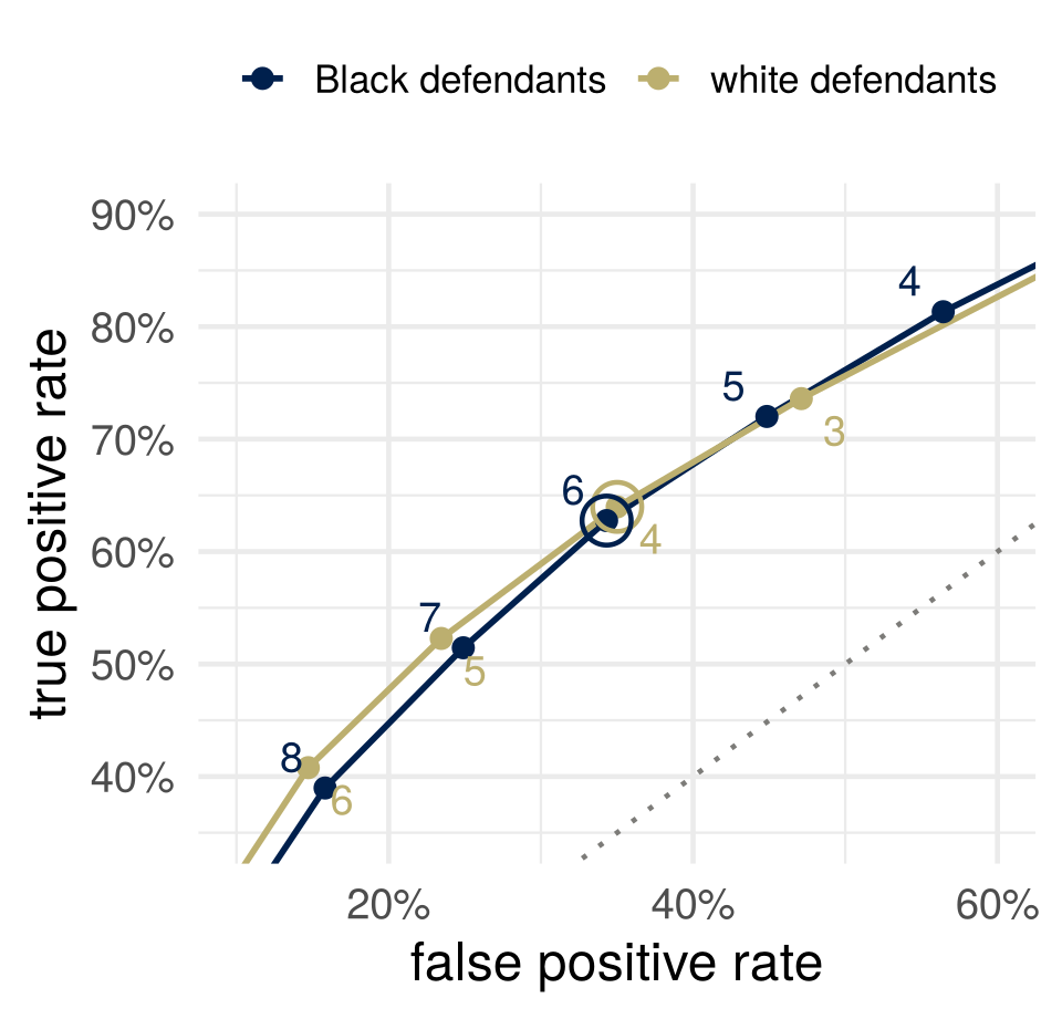
cutoff 5 for both: FPR	45%	23%
FNR	28%	48%
cutoffs 6 and 4: FPR	34%	35%
FNR	37%	36%

A cutoff per group, 6 and 4 (circled), nearly equalizes the error rates. Then the same score means different treatment.

Re-arrest is not reoffending

\(Y = 1\) means a new arrest in Broward County’s records within two years. What we want to know about is reoffending, \(Y^*\). Nobody observes it.

In the fraud checks, a referral counts as correct when the caseworker declines the advance. That outcome is recorded only for requests that were referred, or sampled at random.

Name one way the gap between being arrested and reoffending could differ between the two groups. Which of the four numbers does it move, and which way?

Every rate so far, the base rates included, is a rate of the proxy.

Three views of equality of opportunity

view	the rule	the criterion the book ties to it
narrow	treat similar people similarly, as they are now	calibration by group: the same score means the same thing in every group
middle	treat seemingly dissimilar people similarly when the dissimilarity has causes we should discount	error rate parity, in part: one group should not bear more of the mistakes
broad	organize society so that equal ability and ambition reach equal outcomes	demographic parity, loosely: equal shares, at the decision

The book ties error rate parity to both the middle and the narrow view. ProPublica’s error rates are mostly a middle-view complaint; the predictive values, a narrow-view defense.

Barocas, Hardt and Narayanan (2023), chapter 4, “Equality of opportunity,” pages 81 to 85, and “Connecting statistical and moral notions of fairness,” pages 92 to 97.

A screening test

A test for a disease has sensitivity \(0.9\) and specificity \(0.9\) (TPR \(0.9\), FPR \(0.1\)) in both of two regions. The disease affects \(2\%\) of people in the first region and \(10\%\) in the second.

1. In each region, what share of positive results are correct?
2. In which region is a positive result wrong more often, and who bears that error?
3. The laboratory wants the two shares equal. Can it keep the same error rates in both regions? What does the identity say has to differ?
4. If it moves one region’s cutoff to get there, which criterion has it given up, and who does it owe the explanation to?

Part 5: Where disparities come from

Two worlds, one table

Every criterion in this lecture is a property of the joint distribution of the features, the group, the score and the outcome. With binary \(A\), \(\hat Y\) and \(Y\): eight numbers.

“What observational definitions hide are the mechanisms that created an observed disparity” (the reading, page 72). One table can come from a decision maker who considers group membership out of spite, or from an inequality in society that gives one group an advantage.

For re-arrest, or for the fraud checks: describe two worlds that would give the same table, one where the disparity is the decision maker’s doing and one where it is not.

Barocas, Hardt and Narayanan (2023), chapter 3, “Inherent limitations of observational criteria,” pages 71 to 73.

Lenses this week

• What are we optimizing or predicting? Re-arrest for reoffending; a caseworker’s decline for fraud. Proxies or true outcomes?
• Which comparison gets reported? ProPublica conditioned on the truth, the replies on the flag. The fraud checks report no error rates.
• Who bears the error? A false positive, the person flagged, and detained where the flag decides; a false negative, someone else.
• You have to choose, so choose, and defend it. Equal predictive value or equal error rates. A default chooses too.

Who chose the number?

COMPAS is a commercial product. “Equally accurate in both groups” was the vendor’s headline, and in the sense it meant, equal predictive value, the number is about right.

Who benefited from that being the number that was reported? And would a more competent analyst have chosen a different one?

For next time: bring one decision in which an attribute is used, or deliberately not used, with one route by which it could affect the outcome, and whether that route is fair.