Who counts as a case

Joshua Loftus

Week 5

Part 1: Selection on a common effect

Part 2: Leaving a column out

Part 3: Who is missing

Part 4: Filling in

What you brought

For the dataset you brought: what decided whether someone was in it? Does that depend on the outcome, on something that causes the outcome, or on neither?

Part 1: Selection on a common effect

People offered a place

Cost = need + resources + care-seeking + noise, the four independent. A place for everyone in the top 3% by cost.

Among the people offered a place, are need and resources related? Which way, and why?

The birth weight paradox

US births, 1991:

infants of mothers who smoked: higher risk of low birth weight, and higher infant mortality;
among low-birth-weight infants only: lower mortality for the infants of smokers, relative rate 0.79.

One explanation on offer: smoking is good for babies who are born small.

Hernández-Díaz, Schisterman and Hernán (2006), “The birth weight ‘paradox’ uncovered?”, American Journal of Epidemiology 164(11), 1115–1120, doi:10.1093/aje/kwj275 (the abstract).

Draw it

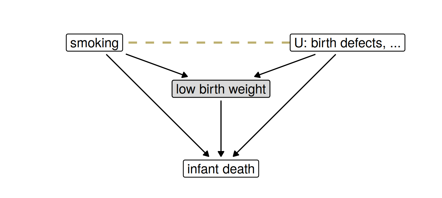
Draw a causal graph in which smoking helps nobody, and the reversal among low-birth-weight infants still appears.

One such graph

Two causal graphs in boxes. Left, all babies: smoking and U (birth defects and other causes) both point into low birth weight, shaded gray; smoking, low birth weight and U all point into infant death. Right, babies born small: low birth weight is gone, smoking and U point into infant death, and a dashed gold line joins smoking and U.

Among babies born small, birth weight is a constant, and smoking and \(U\) are related; among all babies they are not.

Colliders

On a path, a collider is a variable both arrows point into: \(A \to C \leftarrow Y\). The path is blocked until you condition on \(C\), or on something \(C\) causes.

	\(Z\) causes both \(A\) and \(Y\)	\(C\) is caused by both
not adjusted for	an association that is not causal	none
adjusted for	removed	created

Restricting a sample to one value of \(C\) (born small, hired, admitted, offered a place) is conditioning on \(C\).

Barocas, Hardt and Narayanan (2023), Fairness and Machine Learning: Limitations and Opportunities, chapter 5, “Colliders,” pages 112–113, and page 115 of the fairmlbook.org PDF.

Holding the collider fixed

\(A\) and \(Y\) independent, and \(C = Y + A\).

Among people with the same \(C\): \(\; A = C - Y\).

\(\operatorname{Cov}(Y, A \mid C) = \;?\)

With noise

\(A \perp Y\), \(\; C = \beta_Y Y + \beta_A A + \varepsilon\), \(\; \varepsilon\) independent of \((Y, A)\). Take out what \(C\) predicts, with slopes \(\gamma_Y = \operatorname{Cov}(Y, C)/\operatorname{Var}(C)\), \(\gamma_A\) likewise:

\[ \begin{aligned} \operatorname{Cov}(Y - \gamma_Y C,\; A - \gamma_A C) &= \operatorname{Cov}(Y, A) - \frac{\operatorname{Cov}(Y, C)\,\operatorname{Cov}(A, C)}{\operatorname{Var}(C)} \\ &= -\,\frac{\beta_Y\, \beta_A\, \operatorname{Var}(Y)\operatorname{Var}(A)}{\operatorname{Var}(C)} \end{aligned} \]

Adjusting linearly for a common effect relates its causes, sign opposite to \(\beta_Y \beta_A\) here (for jointly normal variables, the covariance given \(C\)). Outside the linear model, sign and size depend on details the graph does not show (Elwert and Winship).

On the last sentence: Elwert and Winship (2014), “Endogenous Selection Bias: The Problem of Conditioning on a Collider Variable,” Annual Review of Sociology 40, 31–53, doi:10.1146/annurev-soc-071913-043455.

Part 2: Leaving a column out

Rows and columns

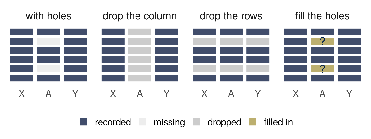
Datasets follow rules for who is a row and for what is a column. A column is absent because the law forbids it, because nobody collected it, or because it was half empty and got dropped. A column with holes forces one of three choices: this part, Part 3, Part 4.

Four small grids of three columns, X, A and Y, and six rows. The first has two holes in column A. The second has column A grayed out: drop the column. The third has the two rows with holes grayed out: drop the rows. The fourth has the two holes filled in gold with question marks: fill the holes.

Predict

\(Y\): job performance, \(N(0, 1)\). \(\; A \in \{0, 1\}\): a group, half each, independent of \(Y\).

\(X = Y + 2A + \varepsilon\): a test score, \(\varepsilon \sim N(0, 1)\) independent. Group 1 gets two points from coaching.

The model may not have \(A\): the law, or a dropped column.

A causal graph: A and Y both point into X.

Predict \(Y\) from \(X\) alone, or from \(X\) and \(A\). Which model is more accurate? Which predicts a bigger gap between the groups?

Two models

group	mean of Y	predicted, X only	predicted, X and A	MSE, X only	MSE, X and A
0	0.00	-0.34	0.00	0.66	0.48
1	0.00	0.31	-0.01	0.64	0.49

Leaving \(A\) out: less accurate in both groups, and a gap between groups whose \(Y\) has the same distribution.

ST313 coursework 2 (2024) and its worked solution: \(A \to X \leftarrow Y\), betaY = 1, betaA = 2: \(\beta_Y = 1\) and \(\beta_A = 2\) in the formula before.

The picture

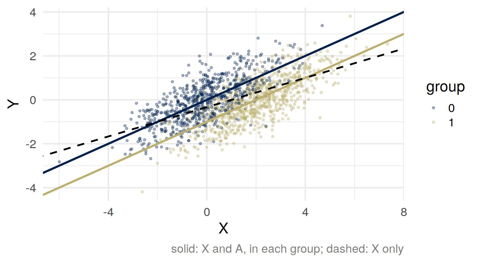
Scatter plot of Y against X for 1,500 people, group 0 in navy and group 1 in gold, the gold cloud shifted right; a navy and a gold line of slope one half, one per group, and a dashed black line of slope one third through both.

True/population values

\(\operatorname{Var}(A) = \tfrac14\), so \(\operatorname{Var}(X) = 1 + 4 \cdot \tfrac14 + 1 = 3\), \(\; E[X] = 1\), \(\; \operatorname{Cov}(X, Y) = 1\).

	\(X\) only	\(X\) and \(A\)
prediction	\(\hat Y = \tfrac13 (X - 1)\)	\(\hat Y = \tfrac12 X - A\)
mean prediction, group 0 and group 1	\(-\tfrac13\) and \(+\tfrac13\)	\(0\) and \(0\)
mean squared error, each group	\(\tfrac23\)	\(\tfrac12\)

The truth: mean \(Y\) is \(0\) in both groups. The coefficient on \(A\) is \(-1\).

Why leave out \(A\)?

Less accurate, more unequal: so why leave out \(A\)?

Direct discrimination (s. 13): less favorable treatment because of a protected characteristic.
Indirect discrimination (s. 19): a provision, criterion or practice applied whatever the characteristic that puts those who share it, this person included, at a particular disadvantage, unless shown to be a proportionate means to a legitimate aim.
A half-empty column dropped in cleaning: no reason stated. The model cannot tell the two apart.

If \(A\) shaped the recorded outcome itself, a model using \(A\) learns that.

Equality Act 2010 (c. 15), sections 13(1) and 19, legislation.gov.uk/ukpga/2010/15.

Adjusting for a collider

Does \(A\) affect \(Y\)?

Compare the groups’ mean \(Y\): \(\; 0\). Right.
The coefficient on \(A\) in lm(Y ~ X + A): \(\; -1\). Among people with the same score, group 1 does worse.

True as a prediction at a fixed score. False as a statement about what changing \(A\) would do.

To predict \(Y\): condition on \(X\) and \(A\). To estimate the effect of \(A\) on \(Y\): do not condition on \(X\).

Part 3: Who is missing

Missing data

\(C = 1\) if \(Y\) is observed: the complete cases. \(X\) is always recorded.

missing completely at random (MCAR): \(C\) independent of \((X, Y)\);
missing at random (MAR): \(C\) independent of \(Y\) given \(X\);
missing not at random (MNAR): neither.

You can check whether \(C\) depends on \(X\). You cannot check, from these data, whether it depends on \(Y\) once \(X\) is accounted for.

Rubin (1976), “Inference and missing data,” Biometrika 63(3), 581–592, doi:10.1093/biomet/63.3.581; van Buuren (2018), Flexible Imputation of Missing Data, 2nd edition, Chapman and Hall/CRC, doi:10.1201/9780429492259, sections 1.2 and 2.2.

Classify, with a direction

A box of paper questionnaires is lost in a flood. Which forms were in the box had nothing to do with their answers.
Older respondents skip the income question more often, and nothing else decides who skips. Age is recorded, and income rises with age.
High earners skip the income question more often, at every age and overall.

MCAR, MAR or MNAR? Is the mean of the recorded incomes too high, too low, or neither?

Complete-case bias

\[ \begin{aligned} E[Y \mid C = 1] &= \frac{E[YC]}{P(C = 1)} \\ \operatorname{Cov}(Y, C) &= E[YC] - E[Y]\,P(C = 1) \\ E[Y \mid C = 1] - E[Y] &= \frac{\operatorname{Cov}(Y, C)}{P(C = 1)} \end{aligned} \]

MCAR: \(0\). Fewer cases, so more variance; no bias.
MAR: \(\operatorname{Cov}(Y, C) = \operatorname{Cov}\big(E[Y \mid X],\; P(C = 1 \mid X)\big)\): a bias, unless the two are uncorrelated.
MNAR: not computable from the data. Argue its sign.

Compute

Two age groups, equally common. Mean income 40 in the younger, 60 in the older (thousands).

The younger answer the income question with probability 0.8, the older with probability 0.4. Within each group, answering is unrelated to income.

The true mean? The mean among those who answered? Check with the formula.

When the complete cases are enough

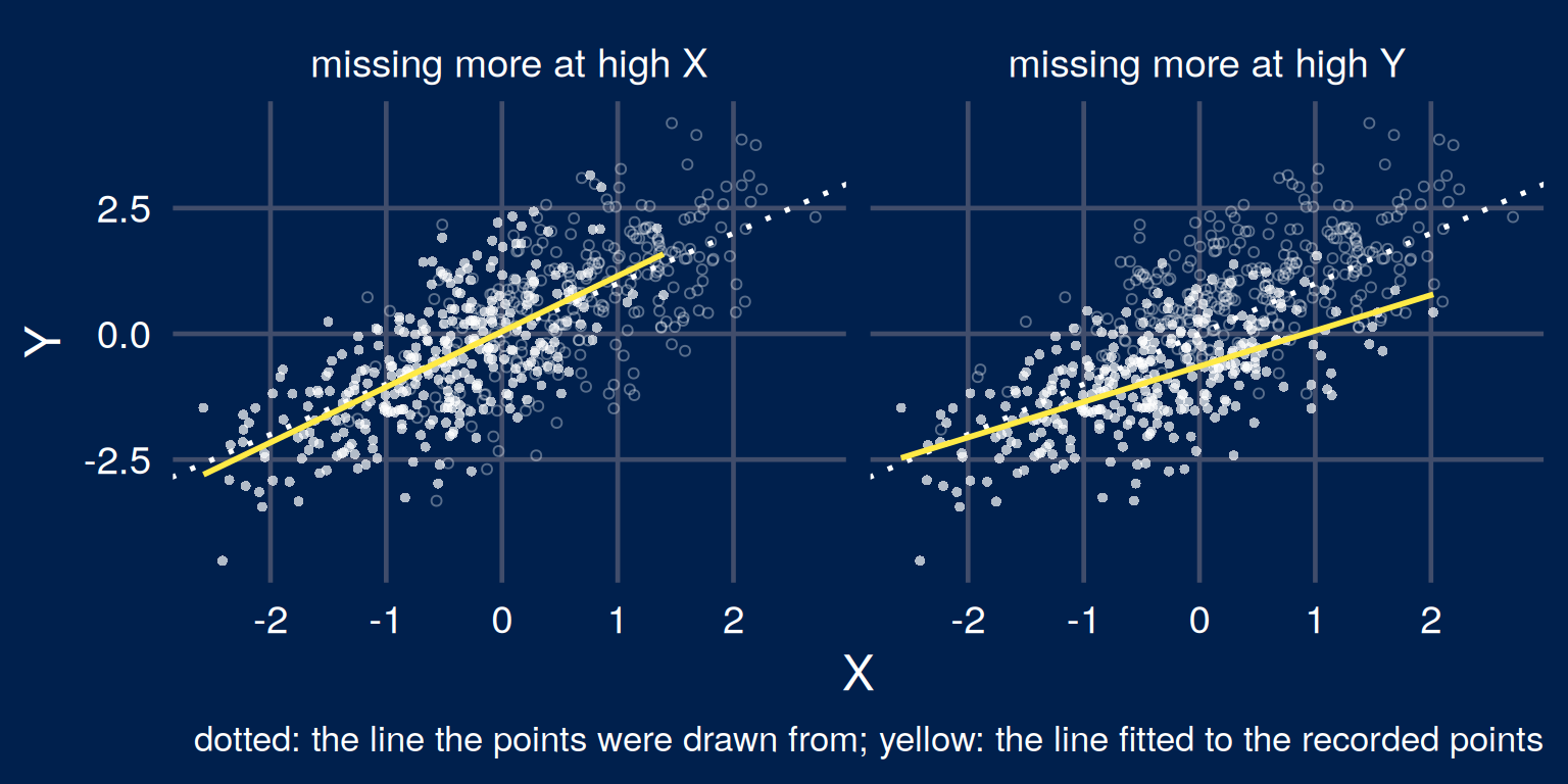
Two panels of simulated points with a dotted line of slope one, the line they were drawn from. Left, missing more often at high X: the solid line fitted to the recorded points lies on the dotted line. Right, missing more often at high Y: the fitted line is flatter.

Missing on \(X\) only: \(E[Y \mid X, C = 1] = E[Y \mid X]\), a correct line survives. Missing on \(Y\) given \(X\): it need not; here it flattens.

Inverse probability weighting

\(e(X) = P(C = 1 \mid X) > 0\). Under MAR:

\[ E\left[\frac{C\,Y}{e(X)}\right] = E\left[\frac{E[C \mid X]\;E[Y \mid X]}{e(X)}\right] = E\big[E[Y \mid X]\big] = E[Y] \]

Income example: \(\tfrac12 (0.8)(40)/0.8 + \tfrac12 (0.4)(60)/0.4 = 50\).

Each respondent stands for \(1/e(X)\) people like them. Horvitz and Thompson’s estimator, with the chance of answering in place of the chance of being sampled; the same weights as inverse propensity weighting for a treatment, with “answered” in place of “treated”.

Horvitz and Thompson (1952), “A Generalization of Sampling Without Replacement from a Finite Universe,” Journal of the American Statistical Association 47(260), 663–685, doi:10.1080/01621459.1952.10483446. The same weights for people lost to follow-up: Hernán and Robins, Causal Inference: What If, section 8.5.

Missing by construction

Bail: whether a defendant fails to appear is recorded only if the judge released them. If the judge used things the record does not have, and they predict the outcome, the detained are those expected to do worst given the record.

“the observed outcomes are themselves a consequence of the existing choices of the human decision-makers”

A study in the file drawer, missing because of its own \(z\)-value; a post that did not reach your feed, because it was not extreme enough.

Lakkaraju, Kleinberg, Leskovec, Ludwig and Mullainathan (2017), “The Selective Labels Problem,” Proceedings of the 23rd ACM SIGKDD International Conference on Knowledge Discovery and Data Mining, 275–284, doi:10.1145/3097983.3098066; the quotation is from the abstract, page 275.

Part 4: Filling in

Filling in

Ways to fill a hole, worked through in the class:

the mean of the recorded values: mean imputation;
a regression prediction from the recorded columns: regression imputation;
the person’s last recorded value: last observation carried forward;
several plausible values, each analyzed, the results pooled: multiple imputation (mice);
a column flagging the hole: the indicator method.

An imputation model is an assumption about the values you did not observe, written down where it can be argued with.

van Buuren (2018), Flexible Imputation of Missing Data, 2nd edition, sections 1.3 (ad hoc solutions) and 1.4 (multiple imputation in a nutshell).

The three choices compared

	MSE, A recorded	MSE, A missing	gap, A recorded	gap, A missing
drop the column	0.65	0.68	0.66	0.66
drop the rows	0.50	no prediction	0.02	no prediction
fill in	0.50	0.68	0.03	0.65

\(A\) recorded for half of 5,000 rows, at random. Gap: mean prediction for group 1 minus group 0; the truth is \(0\). Drop the rows: fit on the complete rows, predict only where \(A\) is recorded. Fill in: fit on the completed rows; where \(A\) is missing, average over \(P(A \mid X)\).

Filling in recovers the fit, not the missing information. Where \(A\) is recorded, a model that uses it has no gap; where it is missing, nothing predicts better than \(X\) alone, and the gap is back.

Admitted students

A university’s records cover admitted students only. Admission is by exam grades, with a lower pass mark for applicants from a feeder school. Among applicants, grades and feeder school are unrelated.

Draw the graph and mark what the records condition on. Among admitted students, what association between feeder school and grades do you expect, and why? An analyst concludes that feeder schools produce weaker students. What is wrong?

Lenses this week

Who is in the data? Babies born small; the complete cases; defendants a judge released; people offered a place. And what is recorded about them: the column that was dropped.
You have to choose, so choose, and defend it. Drop the column, drop the rows, or fill in: each depends on something the data do not settle, the graph \(A\) is in, MAR or MNAR. A default makes the choice too, with nobody to defend it.
What can be changed, and how? What things are considered “controlled for” or “held fixed,” and is that realistic? A score held fixed while the group changes. Birth weight held fixed while asking about smoking.

…and why?

In the test-score example, would you leave the group out of the model, or use it? What graph does your answer assume?

For next time: bring one rule or score that sorts people into two groups (admit or reject, flag or clear, treat or not), with the two ways it can be wrong and who pays for each.

Political economy of data

Creating data takes resources. Someone pays to count, to record, and to keep.

What does that mean about which data get created, and which do not?