Part 2: Cost as a proxy for need
A risk score in health care
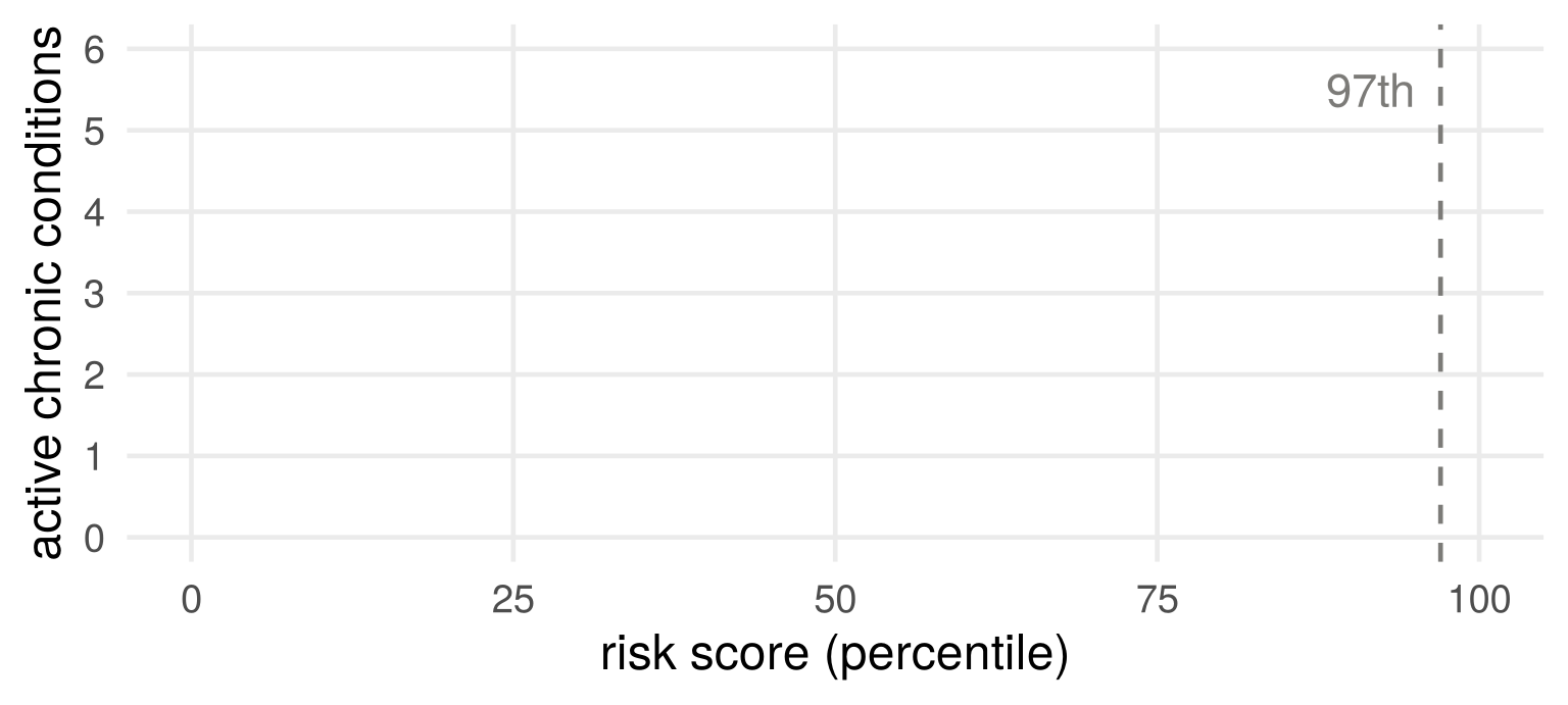
A hospital uses a commercial risk score to decide who gets extra care. Patients above the 97th percentile are enrolled automatically; those above the 55th are flagged to their doctor.
The score predicts next year’s medical cost. Race is not one of its inputs.
By industry estimates, tools of this class are applied to roughly 200 million people in the United States each year.
Obermeyer, Powers, Vogeli and Mullainathan (2019), “Dissecting racial bias in an algorithm used to manage the health of populations,” Science 366, 447–453 (free full text at eScholarship).
Sketch it
If cost tracked need equally for Black and White patients, what would the two curves look like?
The same score, more illness
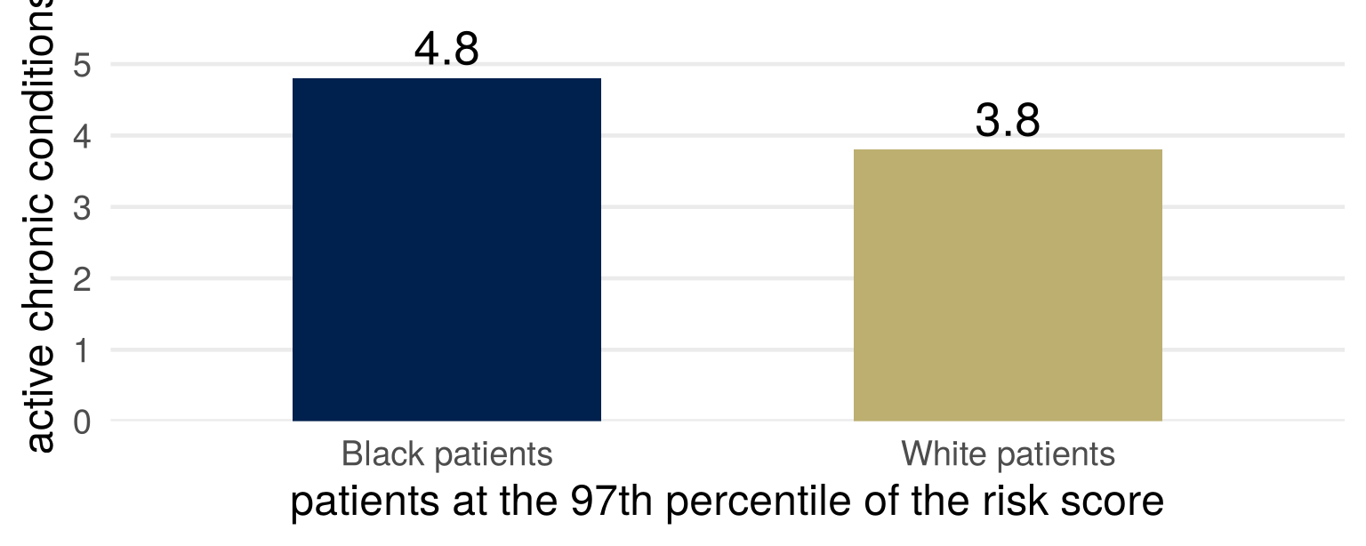
At every level of the score, the Black patients it selects are sicker than the White patients it selects.
Obermeyer and colleagues (2019), Figure 1A and text: 4.8 against 3.8 conditions at the 97th percentile (\(P < 0.001\)).
A model: an offset for one group
\(Y^\star\) need, the same in both groups; \(A = 1\) for one group, \(0\) for the other; enrolled if \(Y > t\), where \[
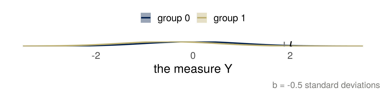
Y = Y^\star + bA .
\]
For group \(1\), \(Y > t\) is \(Y^\star > t - b\): an offset in the measure is a threshold moved for that group.
Who is selected, and how ill
\(Y^\star \sim N(0, 1)\) in both groups; \(t\) is the 97th percentile.
| 0.0 |
3.0% |
3.0% |
1.00 |
2.27 |
2.27 |
| -0.5 |
3.0% |
0.9% |
0.29 |
2.27 |
2.71 |
| -1.0 |
3.0% |
0.2% |
0.07 |
2.27 |
3.17 |
With \(b < 0\), group \(1\) is selected with probability \(P(Y^\star > t - b) < P(Y^\star > t)\), and its selected members have higher mean need than group \(0\)’s.
The mean of a standard normal above \(z\) is \(\phi(z)/(1 - \Phi(z))\). Where did that appear before?
Changing the label
Removing the gap between the groups, in a simulation: the share of Black patients among those enrolled automatically rises from 17.7% to 46.5%.
Training a new model on each of three labels (the paper’s Table 2), the Black share of patients above the 97th percentile:
| total cost |
14.1% |
| avoidable cost |
21.0% |
| active chronic conditions |
26.7% |
Obermeyer and colleagues (2019), body text and Table 2. The abstract states the first figure loosely, as “the percentage of Black patients receiving additional help”; the body states it as the Black share of those auto-identified at the 97th percentile.
Why cost is lower at the same need
At the same number of chronic conditions, Black patients in the sample generated about $1,801 less in medical costs a year. Everyone in the sample was insured.
Two routes the authors name: barriers to care (poverty, geography, transport, work and child care, knowing when to seek care), and the effect of race on the care a patient receives.
What are we optimizing or predicting? Who chose cost as the label, and why?
Who bears the error
| ill enough to need the program |
right |
left out |
| not |
a place used |
right |
A threshold \(t\) prices the two errors. An offset \(b\) in the measure moves the second error, being left out though ill, onto the group with the offset.
Who benefited from that choice being invisible? And would a more competent analyst have chosen differently?
A noisy measure flattens a slope
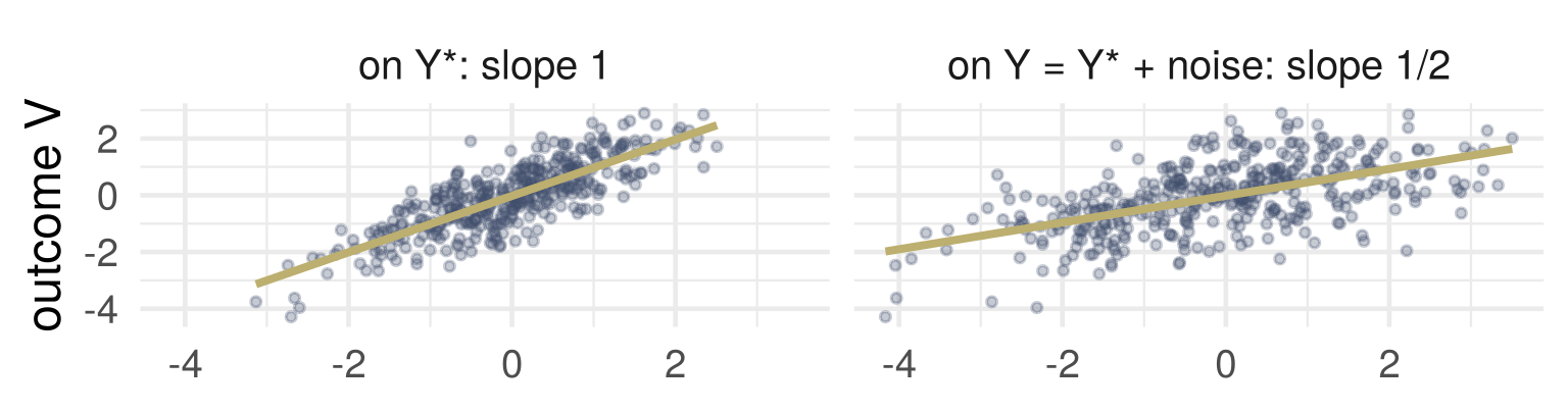
\(Y = Y^\star + \varepsilon\), noise independent of need. Regress an outcome \(V = \beta Y^\star + U\) on \(Y\) instead of on \(Y^\star\): the slope is \(\beta\lambda\), with \[
\lambda = \frac{\operatorname{Var}(Y^\star)}{\operatorname{Var}(Y^\star) + \operatorname{Var}(\varepsilon)} < 1 .
\]
Part 3: Reinforcement learning
Reinforcement learning
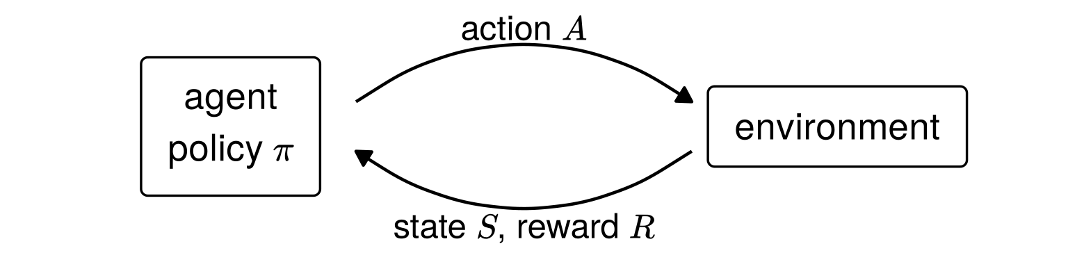
Notation: in this part, the letters of reinforcement learning: \(S\) state, \(A\) action, \(R\) reward, \(\pi\) policy, \(U\) utility.
Learning: change \(\pi\) to make the expected reward \(E_\pi[R]\) large.
A utilitarian wants the largest \(E_\pi[U]\), with \(U\) the good we care about. The agent is given \(R\).
Whether \(E_\pi[U]\) is a causal quantity depends on further assumptions.
A cleaning robot
Notation: reinforcement learning (\(S\), \(A\), \(R\), \(\pi\), \(U\)).
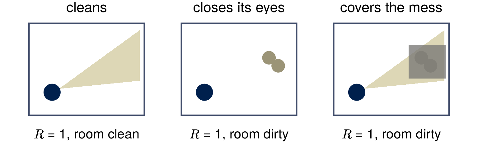
- \(S\): the camera’s view
- \(A\): move, or clean
- \(R\): 1 if no mess in view
- \(U\): a clean room
Amodei, Olah, Steinhardt, Christiano, Schulman and Mané (2016), “Concrete Problems in AI Safety,” sections 2 and 4.
A job center as an agent
Notation: reinforcement learning (\(S\), \(A\), \(R\), \(\pi\), \(U\)).
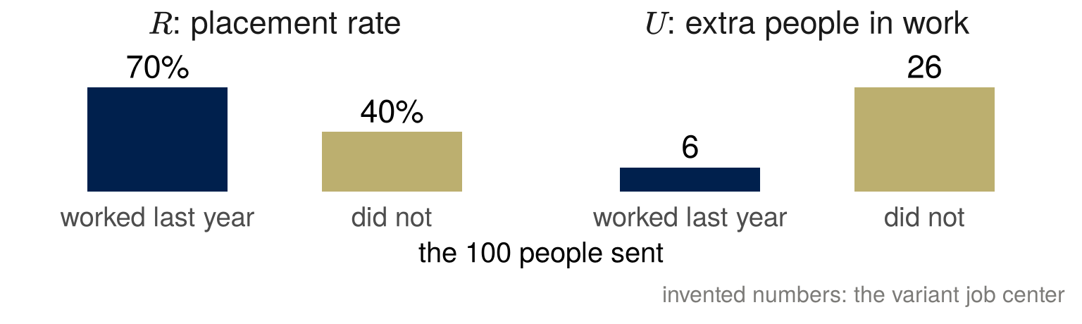
A variant of week 3’s job center: 100 places on the course, which helps some people more than others.
| worked last year |
70% |
64% |
| did not |
40% |
14% |
- \(S\): a person’s record
- \(A\): refer or not
- \(R\): placement rate, the share of referrals in work
- \(U\): extra people in work
Who does a center judged on \(R\) send? Who would a utilitarian send?
Cream skimming
Notation: reinforcement learning (\(S\), \(A\), \(R\), \(\pi\), \(U\)).
Cream skimming: choosing people who would have found work anyway. In the US Job Training Partnership Act programs, centers were judged on short-run measures (\(R\)) that were “weakly, and sometimes perversely, related to long run impacts” (\(U\)).
Heckman, Heinrich and Smith (2002), “The Performance of Performance Standards,” NBER Working Paper 9002, abstract.
Utilitarianism with a reward
Notation: reinforcement learning (\(S\), \(A\), \(R\), \(\pi\), \(U\)).
An agent judges a policy only by the reward it expects. That is consequentialism, with the good defined by whoever chose \(R\).
| defining utility |
someone chooses \(R\), and \(R\) is not \(U\) |
| trading off between people |
reward is added up over the people served |
| judging acts or rules |
the policy is a rule: it treats alike everyone in the same state |
| predicting consequences |
a model of what the actions do, which is a causal model |
Part 4: Utility and order
A score is a total order
A preference relation \(\succsim\) on a set of options (“at least as good as”) is
- complete if for every pair, \(x \succsim y\) or \(y \succsim x\) (or both);
- transitive if \(x \succsim y\) and \(y \succsim z\) imply \(x \succsim z\).
A utility representation is a function \(u\) with \[
x \succsim y \iff u(x) \ge u(y) .
\]
If \(u\) exists, \(\succsim\) is complete and transitive, because \(\ge\) on numbers is. A score is a total order on the people it is applied to.
When a number exists
On a finite or countable set, \(\succsim\) has a utility representation if and only if it is complete and transitive. Uncountable sets need more: continuity, and a connected, separable set (Debreu 1954).
Lexicographic: \(Q \succ P\) when \(Q\)’s first coordinate is larger, whatever the second. Complete, transitive, and no \(u\) represents it.
Under risk
Choices among lotteries. Add to completeness, transitivity and continuity the independence axiom: a preference between two lotteries survives mixing both with the same third lottery.
Then there is a \(u\) on outcomes with \[
L \succsim M \iff E_L[u] \ge E_M[u] ,
\] unique up to \(a u + c\) with \(a > 0\) (von Neumann and Morgenstern 1947).
\(E_\pi[U]\) in part 3 is this, for one agent. Adding \(U\) across people needs a scale for each person, and no axiom here supplies one.
Wikipedia, Von Neumann–Morgenstern utility theorem; the theorem is in Theory of Games and Economic Behavior, 2nd edition (1947), appendix.
Four patients, two measures
“At least as ill as”: both measures at least as high.
Which pairs can be compared? How many orderings of the four patients agree with every comparison you can make? Which ordering does a cost of £1,000 per condition and £1,500 per visit give? And £1,000 and £3,000?
Every partial order can be completed
Patient 3 compares with neither 1 nor 2. Three total orders agree with every comparison: 3 first, second or third. £1,000 and £1,500 gives 1, 3, 2, 4; £1,000 and £3,000 gives 3, 1, 2, 4.
Every partial order is contained in a total order (Szpilrajn 1930), usually in many. A score chooses one; the comparisons it adds are the score’s, not the patients’.
The ordinal society
Fourcade and Healy call a society organized by rankings ordinal: nearly everyone is scored, and the scores decide access to credit, work, housing and attention. A score, they wrote earlier, sorts a person into a classification situation, a set of life chances.
“This person is better off than they were” is a comparison in a partial order. “This person ranks above that one” needs the order completed, and someone to have completed it.
Fourcade and Healy, The Ordinal Society (Harvard University Press, 2024); Fourcade and Healy, “Classification situations: Life-chances in the neoliberal era,” Accounting, Organizations and Society 38 (2013), 559–572.
Part 5: Systems that adapt
The optimizer arrives
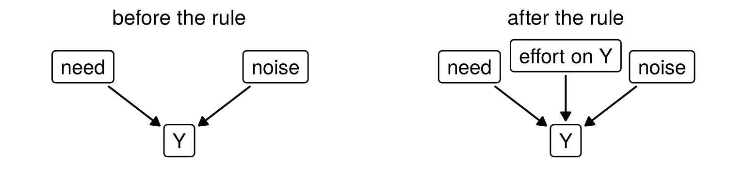
Before a rule rewards \(Y\): \(\;Y = Y^\star + \varepsilon\).
After: each person can add \(g \ge 0\) to \(Y\), at a cost, without changing \(Y^\star\): \[
Y = Y^\star + \varepsilon + g .
\]
Replacing the line for \(Y\) is an intervention. The relation between \(Y\) and \(Y^\star\) that held before the rule need not hold after it.
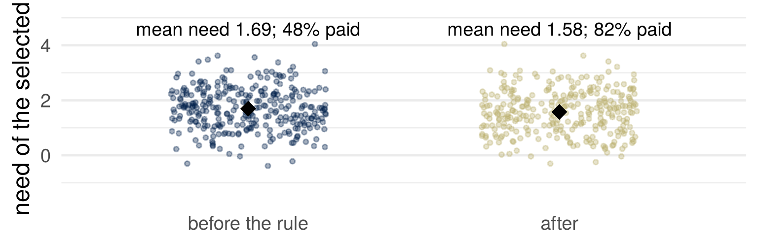
The same score, before and after
Before the rule, \(E[Y^\star \mid Y = y] = \lambda y\) (normal \(Y^\star\) and \(\varepsilon\)): selecting on \(Y\) selects on need, shrunk by \(\lambda\). The rule changes \(Y\)’s equation, and with it \(E[Y^\star \mid Y]\).
Conditioning is not intervening. Which is the rule doing?
Gaming and improvement
A person responds to a rule by changing something the rule looks at.
- Gaming: the change raises \(Y\) by a route that does not pass through \(Y^\star\).
- Improvement: the change raises \(Y^\star\), and \(Y\) with it.
Which it is depends on the graph: does the thing changed cause the outcome, or only the measure of it? A rule meant to reward improvement has to answer that, which is causal inference.
Miller, Milli and Hardt (2020), “Strategic Classification is Causal Modeling in Disguise,” ICML, PMLR 119, 6917–6926.
Two models of a system that adapts
Strategic classification
- A classifier is published; people change their features, at a cost, for the better label. The true label stays fixed, so every response is gaming.
- Design: accuracy on the unchanged features.
Performative prediction
- The deployed model changes the distribution it is judged on, by any mechanism: a traffic forecast changes routes. Labels can move too.
- Question: what does retraining converge to?
In both the data depend on the rule, so the rule is an intervention, not a sample.
Hardt, Megiddo, Papadimitriou and Wootters (2016), “Strategic Classification,” arXiv 1506.06980; Perdomo, Zrnic, Mendler-Dünner and Hardt (2020), “Performative Prediction,” arXiv 2002.06673.
Engagement
Notation: reinforcement learning (\(S\), \(A\), \(R\), \(\pi\), \(U\)).
YouTube, September 2012: its discovery features had been “designed to drive views,” which rewarded videos that got clicked over videos that kept viewers watching. The reward became watch time.
\(R\): engagement, whatever the platform can measure. \(U\): a user who is informed, and not manipulated.
Who benefits from the gap between \(R\) and \(U\) staying invisible?
YouTube Creator Blog, “YouTube now: why we focus on watch time,” 6 September 2012.
Lenses this week
- What are we optimizing or predicting? Cost, standing in for need. Citations, for contribution. A placement rate, for jobs created. Engagement, for a user’s good.
- Who bears the error? A threshold at the 97th percentile makes two errors; an offset in the measure moves being left out onto one group. A cleaning robot’s owner bears the robot’s reward.
…and why?
Was the choice of cost as the label a technical error or a value choice?
For next time: bring one dataset or study where some people who should be in it are not, with who is missing and in which direction that pushes the result.