Scores and what they stand for

Important note: this week’s examples include a commercial product and two platforms. Where I say what a company did, the source is the paper or the company’s own statement, linked. Where I say what it should have done, the view is mine, and a well-argued position I think is wrong can still get full marks.

Summary

A score is a number computed about a person and used to decide something about them. The number measures one thing, \(Y\), and is taken to stand for another, \(Y^\star\). The two come apart in three ways: noise, an offset that differs between groups, and a response by the people being measured. A health system’s risk score measured next year’s medical cost and was taken to stand for how ill a patient was; at the same cost, Black patients were sicker, so the score enrolled fewer of them and the ones it did enroll were sicker than the White patients it enrolled. In a model with an offset \(b\) for one group, selecting above a threshold \(t\) on the measure is selecting above \(t - b\) on the thing measured, for that group only.

A score is also a total order: any two people can be compared. A preference relation has a utility representation only if it is complete and transitive, and on a countable set that is also enough. “Better for this person” is a partial order, and every partial order can be completed into a total one, usually in many ways; a score picks one.

Once a score is rewarded, the people and systems it is applied to act on the score. That changes the equation for \(Y\), an intervention, and what \(Y\) says about \(Y^\star\) afterward is not what it said before. Strategic classification and performative prediction are two formal versions of this. Reinforcement learning says the same thing in other letters: an agent is given a reward \(R\), and the good we care about is a utility \(U\).

Scores

Citation counts

Week 1 followed studies through one filter: of the tests that were run, the ones with \(p < 0.05\) were the ones that reached print. The same filter operates further down the pipeline. De Vries and colleagues (2018) took 105 trials of antidepressants that drug companies had registered with the US Food and Drug Administration, which classified 53 as positive and 52 as negative or questionable, and followed them into the literature.

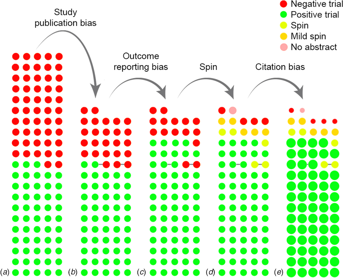
Of the 105 trials, 77 were published: 98% of the positive trials and 48% of the negative ones. Ten negative trials appeared positive in print after an unfavorable outcome was dropped or a secondary outcome promoted to primary. Of the 77 published, 4 said plainly that the drug had not beaten placebo. And in the literature as cited, positive trials were cited about three times as often as negative ones, 92 citations to 32 on average. Each panel is a selection, and each selection runs the same way. The file-drawer effect turns variance into bias.

A citation count is a score. It is what a researcher’s output is measured by, and it is taken to stand for a contribution to knowledge. The figure shows the two coming apart with nobody doing anything dishonest: at each stage, more of the positive results survive.

What a score does to the people it is applied to

The citation count also does something to the people it measures. A researcher who knows that positive results are published and cited has a reason to find one, and week 1’s p-hacking loop is a way of finding one. Last week’s lecture put it in one sentence: what a score does to the people who write for it is a different mechanism from selection.

The usual name for this is Goodhart’s law. Charles Goodhart, a Bank of England economist, wrote in 1975 that “Any observed statistical regularity will tend to collapse once pressure is placed upon it for control purposes.” He was writing about monetary targets: once the Bank tried to control a money-supply measure that had predicted inflation, the measure stopped predicting it. The wording most people know is Marilyn Strathern’s, from a 1997 paper on auditing British universities: “When a measure becomes a target, it ceases to be a good measure.” (Both as cited in the Wikipedia article, which you were asked to skim.) Donald Campbell said something close in 1979 about social indicators, and the two are often quoted together.

Manheim and Garrabrant (2018) sort the ways this happens into four. Their regressional case is the one the next section derives: a proxy that is the goal plus noise overstates the goal wherever the proxy is large. Their causal case is the one this week’s title is about: the regulator’s own action on the proxy breaks the relation between proxy and goal. The other two, extremal (an optimizer pushes the system into a region where the old relation does not hold) and adversarial (someone with other aims acts on the measure), are named here and not developed.

Measured and intended

Write \(Y\) for the outcome a system measures and \(Y^\star\) for the one it was meant to measure: the one we would use if we could. In a regression \(Y\) is the response; in a classifier it is the label; in a reward signal it is the number the agent is given.

\(Y\), measured	\(Y^\star\), intended
citations	contribution to knowledge
\(p < 0.05\)	a true effect
a job center’s placement rate	people in work because of it
a patient’s medical cost	how ill the patient is
a video’s views	a viewer informed, or entertained, on their own terms

The two differ by three routes, and the rest of these notes take them in turn.

1. Noise. \(Y = Y^\star + \varepsilon\), with \(\varepsilon\) unrelated to anything else. A noisy measure is still right on average, but anything estimated from it is attenuated.
2. An offset that differs between groups. \(Y = Y^\star + bA\), with \(A\) a group and \(b \ne 0\). The measure is right on average for one group and off by \(b\) for the other, and selecting on it selects the groups differently.
3. A response to being measured. Once \(Y\) is rewarded, the people and systems it is applied to act on \(Y\) itself. The equation for \(Y\) changes.

The first lens asks about every row of the table: what are we optimizing or predicting? The answer “cost” or “views” is correct and incomplete. The next question is what the number was taken to stand for, and who decided that it could.

Cost as a proxy for need

A risk score in health care

Obermeyer, Powers, Vogeli and Mullainathan (2019) studied a commercial risk score at a large academic hospital. The score was used to decide which patients got extra care. Patients above the 97th percentile of the score were enrolled in a care-management program automatically; patients above the 55th were flagged to their doctor. The score was a prediction of each patient’s medical costs in the coming year, and race was not one of its inputs. By industry estimates, the authors write, tools of this class are applied to roughly 200 million people in the United States each year.

The sample was patients in primary care at the hospital from 2013 to 2015: 6,079 Black patients and 43,539 White patients, counted over 11,929 and 88,080 patient-years. A patient-year is one patient’s data for one calendar year. The authors could see each patient’s score and their health records.

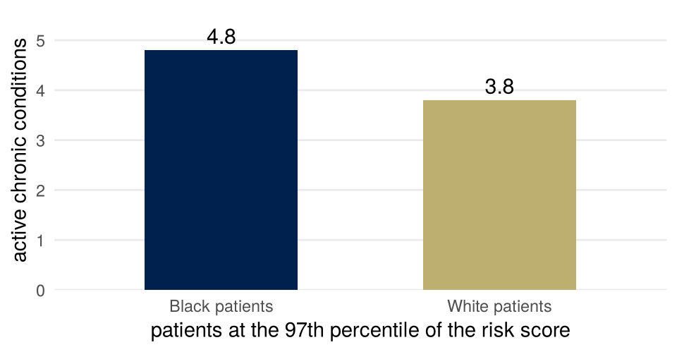
At a given score, Black and White patients cost about the same in the following year, which is what a cost model should deliver. At a given score, Black patients were sicker. The paper’s Figure 1A plots the number of active chronic conditions against the score’s percentile, one curve per group, and the Black curve lies above the White one everywhere. At the 97th percentile, the automatic-enrollment point, Black patients averaged 4.8 active chronic conditions and White patients 3.8, 26% more.

Why? At the same number of chronic conditions, Black patients in the sample generated about $1,801 less in medical costs a year, and everyone in the sample was insured. The authors name two routes. Barriers to care: poverty, geography, transport, the demands of work and child care, and knowing when to seek care, all of which reduce spending at a given level of illness. And the effect of race on the care a patient receives once they are seen; the paper cites a trial in which Black patients took up more preventive care from a Black doctor. Either way, cost measures need with an offset that depends on race.

The authors cannot change the hospital’s tool, so they simulate what removing the gap would do. The share of Black patients among those enrolled automatically would rise from 17.7% to 46.5%. Separately, they trained new models on three labels. With total cost as the label, Black patients were 14.1% of the highest-risk group (the 97th percentile and above); with avoidable cost, 21.0%; with the number of active chronic conditions, 26.7%. The label is the choice, and the paper is about what that one choice did.

The paper’s abstract describes the first figure as “the percentage of Black patients receiving additional help,” which is not what was computed; the body gives the Black share of patients auto-identified at the 97th percentile. A paper about a loosely specified target whose abstract loosely specifies its own number is the first lens applied to the paper that teaches it. Read the body.

A model: an offset for one group

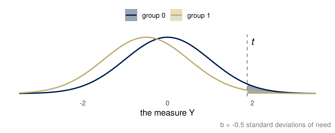
Take need \(Y^\star\) to have the same distribution in both groups, and let \(A = 1\) for one group and \(0\) for the other. The measure is \[ Y = Y^\star + bA , \] and the program enrolls everyone with \(Y > t\). For group \(0\) that is \(Y^\star > t\). For group \(1\) it is \(Y^\star + b > t\), or \(Y^\star > t - b\). An offset of \(b\) in the measure is a threshold moved by \(-b\) for that group. With \(b < 0\), as in the paper, group \(1\) has to be iller to be enrolled.

Two things follow, and both are in the paper’s data.

Who is selected. Group \(1\) is enrolled with probability \(P(Y^\star > t - b)\) and group \(0\) with probability \(P(Y^\star > t)\). With \(Y^\star \sim N(0, 1)\) and \(t\) the 97th percentile, \(t = 1.88\):

offset \(b\)	selected, group 0	selected, group 1	ratio	mean need of the selected, group 0	mean need, group 1
0.0	3.0%	3.0%	1.00	2.27	2.27
-0.5	3.0%	0.9%	0.29	2.27	2.71
-1.0	3.0%	0.2%	0.07	2.27	3.17

An offset of half a standard deviation cuts group \(1\)’s chance of enrollment to less than a third of group \(0\)’s. The ratio falls fast because the threshold is in the tail, where the normal density drops quickly: the same offset at the median would change the two shares by much less.

How ill the selected are. The mean of a standard normal variable given that it exceeds \(z\) is \[ E[Y^\star \mid Y^\star > z] = \frac{\phi(z)}{1 - \Phi(z)} , \] the inverse Mills ratio from week 1, where it gave the expected size of an estimate that survived the significance filter. Here it gives the mean need of the enrolled in each group: \(z = t\) for group \(0\) and \(z = t - b\) for group \(1\). Since the ratio increases in \(z\), the enrolled members of group \(1\) are iller on average than the enrolled members of group \(0\), by about half a standard deviation in the second row of the table. That is the paper’s Figure 1A: at every score, and in particular at the 97th percentile, the Black patients the score selected had more chronic conditions than the White patients it selected.

This is a bias, and more data does not touch it. A larger sample estimates the offset more precisely and enrolls the same people.

The model assumes need has the same distribution in both groups. In the paper’s sample it does not (Black patients were on average sicker), which is why the paper’s shares are what they are rather than the table’s; the direction of both effects is the same. The model also assumes the offset is the same for everyone in group \(1\), when in the paper it comes from barriers that vary from person to person. Read the table as a mechanism, not as the hospital’s numbers.

Who bears the error

A threshold makes two kinds of mistake. A patient can be enrolled without needing the program, which uses a place and the program’s time. A patient can be left out while needing it, which costs the patient. Setting \(t\) at the 97th percentile rather than the 90th says how the hospital priced the two: fewer places used, more people left out.

	enrolled	not enrolled
ill enough to need the program	right	left out
not	a place used	right

The offset moves the second error onto one group. For a Black patient at the enrollment threshold, the score says “not ill enough” at a level of illness at which it says “enrolled” for a White patient. The price of an error is paid by the person it falls on, and the offset decides who that is. The fourth lens asks who bears the error; here the answer is the group whose costs were lower at the same need.

Then the standing question. Who benefited from that choice being invisible? The tool predicted cost, and for a program whose aim was to cut costs that was a defensible label, which the authors say. Nobody had to decide that cost stood for need; the label did it for them. And would a more competent analyst have chosen differently? The paper’s own answer is yes, in a specific way: the program mostly prevents acute episodes in people with chronic illness, so avoidable cost or the number of chronic conditions would have measured what the program was for, and the authors worked with the manufacturer to change the label.

A noisy measure flattens a slope

The first of the three routes is noise. Let \(Y = Y^\star + \varepsilon\), with \(\varepsilon\) independent of \(Y^\star\) and of everything else, mean zero and variance \(\sigma_\varepsilon^2\). Suppose an outcome \(V\) depends on need, \(V = \beta Y^\star + U\), with \(U\) independent noise. Someone with the measure but not the need regresses \(V\) on \(Y\). The population slope is \[ \frac{\operatorname{Cov}(V, Y)}{\operatorname{Var}(Y)} = \frac{\operatorname{Cov}(\beta Y^\star + U,\; Y^\star + \varepsilon)}{\operatorname{Var}(Y^\star) + \sigma_\varepsilon^2} = \frac{\beta \operatorname{Var}(Y^\star)}{\operatorname{Var}(Y^\star) + \sigma_\varepsilon^2} = \beta\lambda , \] because every cross-covariance between the noises and \(Y^\star\) is zero. The factor \[ \lambda = \frac{\operatorname{Var}(Y^\star)}{\operatorname{Var}(Y^\star) + \sigma_\varepsilon^2} \] is between \(0\) and \(1\). It is called the reliability of the measure: the share of its variance that is need rather than noise. The slope is attenuated toward zero by \(\lambda\), however large the sample. Noise in the outcome \(V\) does nothing of the kind: it widens the interval around the slope and leaves its center alone. This is week 2’s sentence again, more data, the same wrong answer, with variance in the measure turned into bias in the slope.

`geom_smooth()` using formula = 'y ~ x'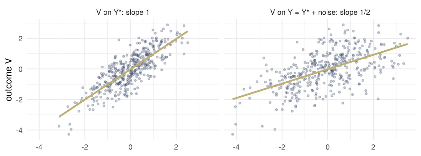

The figure has \(\operatorname{Var}(Y^\star) = \sigma_\varepsilon^2 = 1\), so \(\lambda = 1/2\). The same algebra with \(V\) replaced by \(Y^\star\) itself gives the regression of need on the measure, \[ E[Y^\star \mid Y] = \lambda Y \] when \(Y^\star\) and \(\varepsilon\) are jointly normal with mean zero. A patient whose measure is two standard deviations above average is expected to be one above average in need. Selecting the top 3% by the measure selects people whose need is high, but less high than their measure says, by the factor \(\lambda\). Manheim and Garrabrant call this the regressional version of Goodhart’s law: pick the largest values of a proxy and you have picked its noise along with its signal. This is where the week’s two routes meet: an offset biases the slope’s location for one group, and noise biases its size for everyone.

Reinforcement learning

Notation: this section uses the letters of reinforcement learning: \(S\) state, \(A\) action, \(R\) reward, \(\pi\) policy, \(U\) utility.

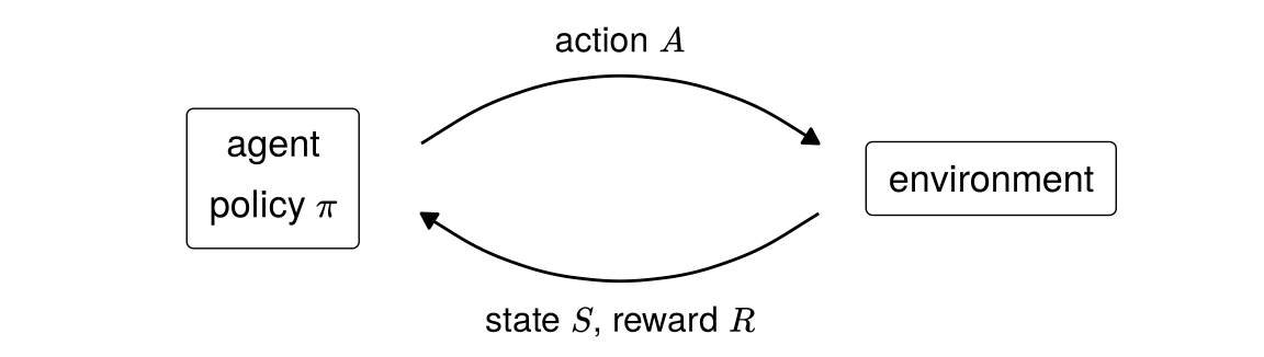
An agent observes a state \(S\), takes an action \(A\), and receives a reward \(R\). A policy \(\pi\) is a rule that chooses the action from the state, \(A = \pi(S)\), and learning means changing the policy to make the expected reward, \(E_\pi[R]\), large, where \(E_\pi\) is the expectation when the agent acts by \(\pi\). The utility \(U\) is what we care about. A utilitarian would choose the policy whose expected utility \(E_\pi[U]\) is largest. The agent is given \(R\) instead, because \(R\) can be measured and \(U\) often cannot: in the job center below, \(U\) needs what would have happened without the course. \(R\) and \(U\) can come apart. In the letters of the rest of these notes, \(R\) is \(Y\) and \(U\) is \(Y^\star\).

Amodei and colleagues (2016) use a cleaning robot as a running example. In these letters, the state is what the robot’s camera shows, the actions are where to move and whether to clean, and the utility is a clean room. If the reward is for not seeing any mess, the robot can earn it by closing its eyes, or by covering the mess with something it cannot see through.

Warning in geom_rect(data = room, aes(xmin = 0, xmax = 10, ymin = 0, ymax = 8), : All aesthetics have length 1, but the data has 3 rows.
i Please consider using `annotate()` or provide this layer with data containing
  a single row.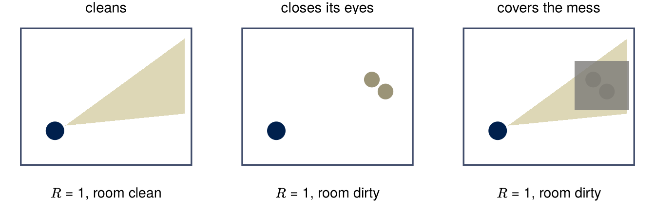

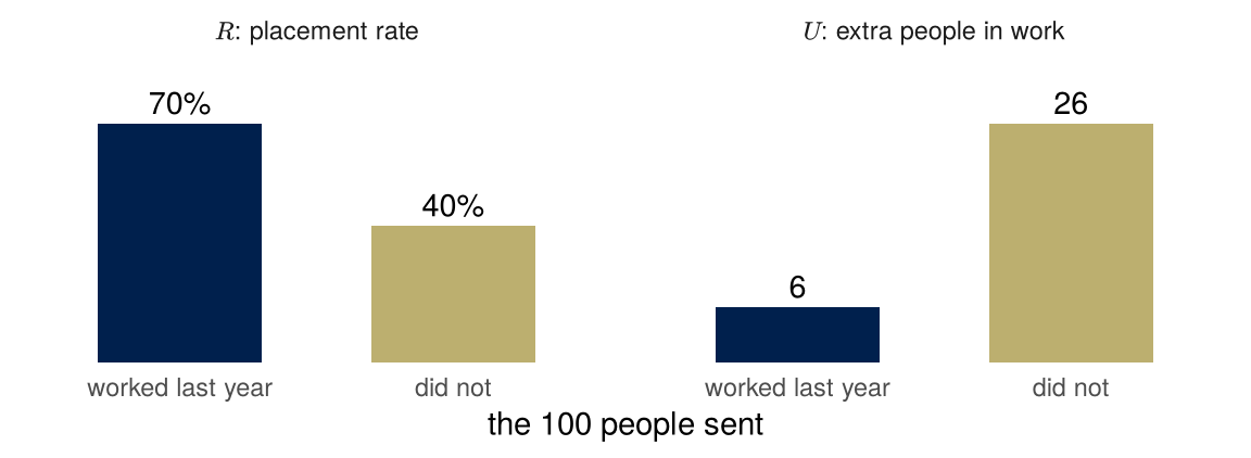
Now a variant of week 3’s job center, with 100 places on the course, which helps some people more than others. Of people who worked last year, 70% are in work six months later if they take the course and 64% if they do not; of people who did not work last year, 40% and 14%. The state is a person’s record, the action is to refer or not, and the center is judged on the share of the people it refers who are in work, its placement rate. That rate is its reward. Referring 100 people who worked last year earns a rate of 70% and puts 6 more people in work, on average, than would be in work without the course. Referring 100 who did not earns 40% and puts 26 more in work. A center judged on its placement rate refers the first group; a utilitarian counting the jobs the course creates refers the second, and so serves the people who need the course most.

Choosing people who would have done well anyway is called cream skimming. Heckman, Heinrich and Smith (2002) studied it in US job-training centers funded under the Job Training Partnership Act, which were judged partly on employment rates. They found the short-run measures “weakly, and sometimes perversely, related to long run impacts.” They also found that cream skimming made little difference to the programs’ efficiency, in either direction, unlike the invented numbers above, and concluded: “Opposition to cream skimming must come on equity grounds.” Equity here is about who is served; efficiency is about the total.

Each of the four difficulties of utilitarianism from week 3 becomes a choice someone makes in building such an agent. Defining utility becomes choosing \(R\), a measurable stand-in for \(U\), and in both examples the two come apart. Trading off between people becomes adding the reward up over the people the agent serves; the placement rate counts only the people referred. Judging acts or rules becomes choosing a policy, a rule that treats alike everyone in the same state. Judging each action on its own and judging the rule can give different answers: when a rule has to treat different situations alike, as a model that sees only a few variables about each person does; when places are limited, so that one referral uses a place another person could have had; and when people respond to the rule itself. Predicting consequences becomes choosing a model of what the actions do, which is a causal model.

Is \(E_\pi[U]\) a causal quantity? It can be read as one, the expected utility if the agent’s actions were set by \(\pi\), but that reading needs assumptions beyond last week’s. An intervention in last week’s sense sets a variable for everyone in a population. Here one agent follows a rule. The people and systems it acts on may respond to what it does, sometimes adversarially, and what happens to one of them can depend on what was done to others. Causal reinforcement learning, a subfield surveyed by Deng, Jiang, Long and Zhang (2023), brings causal models into reinforcement learning.

These letters clash with the ones used for prediction, which most of the course uses.

	prediction	reinforcement learning
\(A\)	sensitive attribute: something a person is	action: something an agent does
\(R\)	risk score, with \(\hat Y = 1\{R \ge t\}\)	reward
\(U\)	unobserved variable	utility
\(S\), \(\pi\)	not used	state, policy

If you read about reinforcement learning you will meet these letters with these meanings. New letters invented for this course would teach a convention nobody else uses. Two rules are enough. Material that uses the reinforcement-learning letters says so in one line at the top, as this section does. And the two sets of letters are never mixed inside one diagram or one derivation. A classifier described as an agent takes its prediction \(\hat Y\) as its action, which reinforcement learning would write as \(A\). Mixing the two there would give \(A\) two meanings in one line.

Utility and order

A score is a total order

Before anything is said about what a score measures, it does one thing: it puts the people it is applied to in order. Any two of them get a number, so any two can be compared, and if the first is above the second and the second above the third, the first is above the third.

The language for this is decision theory’s. A preference relation \(\succsim\) on a set of options reads “at least as good as”. It is

• complete if for every pair of options \(x\) and \(y\), \(x \succsim y\) or \(y \succsim x\) (or both);
• transitive if \(x \succsim y\) and \(y \succsim z\) imply \(x \succsim z\).

A complete and transitive relation is a total preorder, or, when no two distinct options are tied, a total order. A utility representation of \(\succsim\) is a function \(u\) from options to numbers with \[ x \succsim y \iff u(x) \ge u(y) . \]

If \(u\) exists, \(\succsim\) is complete and transitive. Any two numbers compare, and \(\ge\) on numbers is transitive, so the relation \(u\) represents inherits both. That one line is the necessity half of the next theorem, and it says what a score assumes: whatever the score is taken to stand for, the score has ranked everyone against everyone.

When a number exists

The converse is the question. Given a complete and transitive preference, is there always a number?

On a finite or countable set, yes. List the options as \(x_1, x_2, x_3, \ldots\) and define \[ u(x) = \sum_{k:\; x \succsim x_k} 2^{-k} . \] The sum converges, and it adds a term for every option that \(x\) is at least as good as. If \(x \succsim y\) then, by transitivity, every \(x_k\) that \(y\) beats or ties is also beaten or tied by \(x\), so \(u(x) \ge u(y)\). If \(x \succsim y\) fails then, by completeness, \(y \succ x\) strictly; then \(y\)’s sum contains every term of \(x\)’s and also the term for \(y\) itself, which \(x\)’s sum lacks, so \(u(y) > u(x)\). So \(u\) represents \(\succsim\).

On a finite or countable set, \(\succsim\) has a utility representation if and only if it is complete and transitive.

On an uncountable set, complete and transitive are not enough. Order the points of the plane lexicographically: \((a, b) \succ (c, d)\) if \(a > c\), or if \(a = c\) and \(b > d\), as words are ordered in a dictionary. This is complete and transitive. Suppose \(u\) represented it. For each real number \(a\), the points \((a, 1)\) and \((a, 0)\) satisfy \((a, 1) \succ (a, 0)\), so \(u(a, 1) > u(a, 0)\): an interval of positive length on the number line. For \(a < a'\) the interval for \(a'\) lies entirely above the interval for \(a\), since \((a', 0) \succ (a, 1)\). So there would be uncountably many disjoint intervals of positive length in the real line, and there cannot be: each contains a rational number, and there are only countably many of those. No \(u\) exists, continuous or not.

Debreu (1954) gives the extra condition that makes an uncountable case work: if the set of options is connected and separable (the real line, or a region of the plane, is), and \(\succsim\) is complete, transitive and continuous (the set of options at least as good as \(x\), and the set at most as good as \(x\), are both closed), then a continuous utility representation exists. The lexicographic order is not continuous: points just to the left of \((a, 1)\) are all below \((a, 0)\), however close they come.

Under risk

A choice among lotteries, each a probability distribution over outcomes, is the setting of von Neumann and Morgenstern (1947). Their axioms are completeness, transitivity, a continuity condition, and independence: if \(L \succsim M\), then mixing both with the same third lottery \(N\) at the same probability \(p\) preserves the preference, \(pL + (1-p)N \succsim pM + (1-p)N\). Under the four, there is a function \(u\) on outcomes such that \[ L \succsim M \iff E_L[u] \ge E_M[u] , \] the expected utility representation, and \(u\) is unique up to a positive affine transformation: \(au + c\) with \(a > 0\) represents the same preferences and nothing else does.

Two consequences for this course. The agent of the previous section, which chooses the policy with the largest \(E_\pi[R]\), is a von Neumann–Morgenstern agent whose outcomes are rewards; a reward is a utility that someone else wrote down. And the uniqueness clause says what adding utility across people assumes. Each person’s \(u\) is free to be rescaled by any \(a > 0\), so \(u_1(x) + u_2(x)\) depends on which scale each person was assigned, and no axiom about either person’s choices fixes it. Utilitarianism’s second difficulty from week 3, trading off one person’s good against another’s, is this: the total needs a scale for each person that the theory of individual choice does not supply.

Partial orders

Drop completeness. A relation that is reflexive (\(x \succsim x\)), transitive and antisymmetric (if \(x \succsim y\) and \(y \succsim x\) then \(x = y\)) is a partial order: some pairs compare, others do not. Two partial orders matter here.

• Pareto. One state of affairs is at least as good as another if it is at least as good for every person. Most pairs of states do not compare, because most changes help someone and hurt someone else.
• Dominance on several measures. One patient is at least as ill as another if every measure of illness is at least as high.

Take four patients and two measures.

patient	active chronic conditions	emergency visits last year
1	4	2
2	3	2
3	2	3
4	1	1

Patient 1 is at least as ill as patient 2 on both measures, and all three of 1, 2 and 3 are iller than 4. Patient 3 has fewer conditions than 1 and 2 and more visits, so 3 compares with neither.

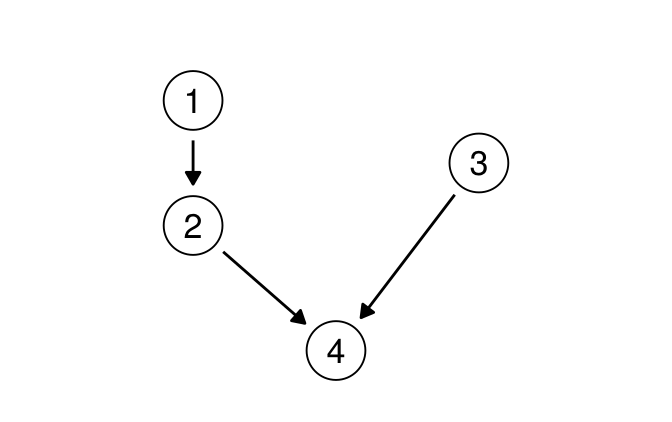
A cost model turns the two measures into one number. At £1,000 per condition and £1,500 per visit, the four patients cost 7,000, 6,000, 6,500 and 2,500, and the order is 1, 3, 2, 4. At £1,000 and £3,000 the costs are 10,000, 9,000, 11,000 and 4,000, and the order is 3, 1, 2, 4. Both orders agree with every comparison the partial order makes. Where the partial order is silent, the weights decide.

Every partial order can be completed

Szpilrajn (1930) proved that every partial order is contained in a total order: one that keeps every comparison of the original and adds comparisons for every pair the original left open. For a finite set this is easy to see, and the number of ways to do it can be counted. The four patients allow three: patient 3 can go first, second or third, and nothing else is free. Four patients with no comparisons at all would allow \(4! = 24\).

A score chooses one of the total orders that contain the partial one, if it respects the partial order at all. The comparisons it adds, 1 against 3 and 2 against 3 above, are not in the measures; they are in the weights, and someone chose the weights. The same holds for any score built from several things: a credit score, a university ranking, a risk score.

This is the shape of the week’s point about scores. “This person is better off than they were” and “this change is better for this person and worse for no one” are statements in a partial order, and they need no weights. “This person ranks above that one” needs the order completed, and completing it is a choice. We can keep the local comparison without granting that everyone can be compared with everyone else; and when a system does compare everyone, the question is who completed the order and how.

The ordinal society

Fourcade and Healy (2024) call a society organized by rankings ordinal: nearly every person and organization is scored, by many systems, and the scores decide access to credit, work, housing and attention. The word points at ranking, and at the French ordinateur, a computer. In an earlier article (Fourcade and Healy 2013) they described how credit scores sort people into what they call classification situations: positions in a market that carry their own prices, terms and life chances, so that the score does not describe a person’s situation so much as assign it. Their examples are US credit markets, where scoring widened access to borrowers once excluded and at the same time drew finer distinctions among them, distinctions that then spread to insurance, housing and employment. They also observe that a score built from past behavior looks fairer than the older exclusions it replaced, such as redlining, while carrying present inequalities forward, and that sorting by merit makes the resulting inequality look deserved.

I read their argument through the previous section. A classification situation is a total order imposed on people whose situations were only partially ordered, and the authors’ concern is with who did the completing and what it did to the people completed.

Systems that adapt

The optimizer arrives

So far the people being measured have done nothing. Now reward the measure. Before the rule, \[ Y = Y^\star + \varepsilon , \] and selecting the people with the highest \(Y\) is conditioning: it picks out a group whose need is high, shrunk by \(\lambda\), because the old relation between \(Y\) and \(Y^\star\) still holds among the people picked. After the rule, each person can add an amount \(g \ge 0\) to their own \(Y\), at some cost, without changing \(Y^\star\): \[ Y = Y^\star + \varepsilon + g . \]

Warning: The `label.size` argument of `geom_label()` is deprecated as of ggplot2 3.5.0.
i Please use the `linewidth` argument instead.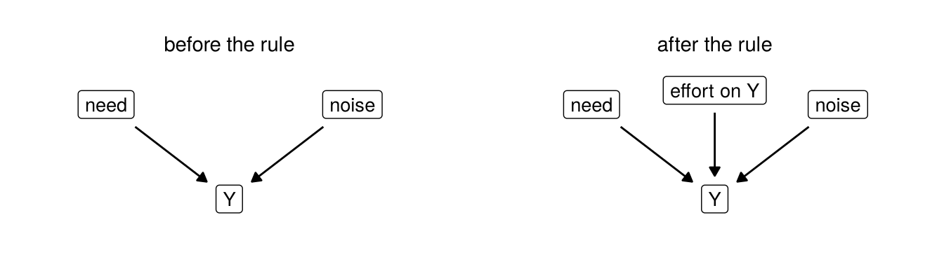

Replacing the line that generates \(Y\) is what week 3 called an intervention: a new assignment for one variable, every other line left alone. The relation between \(Y\) and \(Y^\star\) that held before the rule need not hold after it. Which people it fails for depends on who can pay for \(g\).

A simulation makes the mechanism visible. Ten thousand people, need and noise standard normal, and 300 places for the highest \(Y\). After the rule, the half of the population who can afford it add \(1\) to their \(Y\); ability to pay is independent of need. The 300 places now go mostly to people who paid, and the mean need of the people selected falls.

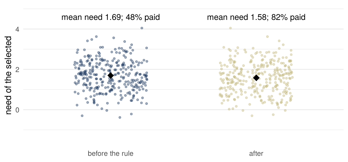
The fall in mean need is modest here, because the people who paid were drawn from the same need distribution as everyone else; what changes most is who the places go to. In the paper’s setting the equivalent would be a hospital that rewards patients, or their doctors, for a high score, after which the score measures who responded to the reward.

   mean_y mean_need 
 3.170883  1.694010 

Two formal versions of a system that adapts are in the reading’s authors’ own work.

Strategic classification (Hardt, Megiddo, Papadimitriou and Wootters 2016). A classifier is published. Each person then changes their features, at a cost that depends on the change, to get the label they want, and the classifier’s accuracy is judged against the features as they were before the change and an underlying target function. The true label is taken as fixed, so every response is gaming, and the design problem is a classifier that stays accurate when everyone games it. The paper gives efficient algorithms for a natural class of cost functions and shows the general problem is hard.

Performative prediction (Perdomo, Zrnic, Mendler-Dünner and Hardt 2020). A prediction that is acted on can change the thing it predicts: a traffic forecast changes which roads people take, and a forecast that a loan will default can make it default. The authors call such predictions performative. The distribution the model is evaluated on depends on the model deployed, by whatever mechanism, and the labels can move along with the features. The question is what retraining on the data a model induces converges to, a model they call performatively stable, and whether that point has low loss. They give conditions under which it does, and show that strategic classification is the special case in which the mechanism is individuals responding to a published rule.

Gaming and improvement (Miller, Milli and Hardt 2020). Whether a response to a rule is gaming or improvement depends on the causal graph. If the feature a person changes causes the outcome, the change improves the outcome, and \(Y^\star\) rises with \(Y\); if it causes only the measure, the change is gaming, the second graph above. A rule meant to reward improvement has to know which, and that is a causal inference problem; the authors show that any procedure for designing such rules has to solve one. Conditioning is not intervening, a third time: the rule intervenes on the people it is applied to, and what they do in response is decided by the graph, not by the rule’s intentions.

Engagement

Notation: this section uses the letters of reinforcement learning: \(S\) state, \(A\) action, \(R\) reward, \(\pi\) policy, \(U\) utility.

A recommender system is an agent. Its state is what it knows about a user, its action is what to show next, and its reward is whatever the platform can measure about the response: a click, a view, time watched, a share. In September 2012 YouTube told its creators that its discovery features had been “designed to drive views,” which rewarded videos that got clicked over videos that kept viewers watching, and that it would rank by watch time instead. A platform’s reward is engagement in some form. A user’s utility is something else: being informed, or entertained, on their own terms, and not manipulated. The gap between the two is where a platform’s revenue is, and that is a reason for nobody inside the platform to close it. Last week’s lens asked which comparison gets reported; this week’s asks what is being optimized, and for whom.

Week 2 showed the selection half of this story: a feed surfaces the most extreme of \(n\) items. This is the optimization half: a feed that ranks by \(R\) changes what gets made, because the people who make it write for the score.

Lenses

What are we optimizing or predicting? Cost, standing in for need. Citations, standing in for a contribution. A placement rate, standing in for jobs created. Views, or watch time, standing in for a viewer’s good. In each case the first word is what the system can measure and the second is what someone wanted; the system’s designer chose the first and the system optimized it.

Who bears the error? A threshold at the 97th percentile makes two errors, a place used on someone who did not need it and a person left out who did, and prices them against each other. An offset in the measure moves the second error onto one group, the one whose costs were lower at the same need. The cleaning robot’s owner bears the difference between the robot’s reward and a clean room; the job seekers a center did not refer bear the difference between its placement rate and the jobs the course would have created.

And why? A measure is chosen because it can be measured. Cost is in the billing system and need is not. Views are counted and a viewer’s understanding is not. The choice is made once, often by a vendor, and afterward nobody has to make it again; the score makes it for them.

For the class

Attenuation, derived

The class derives the slope \(\beta\lambda\) from the covariance algebra above and checks it by simulation, then asks what happens when the noise is in \(V\) instead of in \(Y\), and when \(\varepsilon\) is correlated with \(Y^\star\).

The four patients

The class counts the total orders that extend a partial order by hand, for the four patients and for a fifth patient added to the table, and shows which cost weights pick which order.

Necessity in one line

If \(u\) represents \(\succsim\), then \(\succsim\) is complete and transitive: for any \(x, y\), either \(u(x) \ge u(y)\) or \(u(y) \ge u(x)\), so \(x \succsim y\) or \(y \succsim x\); and \(u(x) \ge u(y) \ge u(z)\) gives \(u(x) \ge u(z)\).

Readings

Required

• Obermeyer, Powers, Vogeli and Mullainathan, Dissecting racial bias in an algorithm used to manage the health of populations (Science 366, 2019, 447–453). Read the body, not only the abstract.
• Barocas, Hardt and Narayanan, Fairness and Machine Learning, chapter 1, Introduction, from “The trouble with measurement” through “Feedback and feedback loops” (pages 7 to 14).
• Skim the Wikipedia article Goodhart’s law.

Optional

• Amodei, Olah, Steinhardt, Christiano, Schulman and Mané, Concrete Problems in AI Safety (2016), sections 2 and 4.
• YouTube Creator Blog, YouTube now: why we focus on watch time (6 September 2012).
• Miller, Milli and Hardt, Strategic Classification is Causal Modeling in Disguise (ICML 2020), section 1.
• Perdomo, Zrnic, Mendler-Dünner and Hardt, Performative Prediction (ICML 2020), section 1.
• Jacobs and Wallach, Measurement and Fairness (ACM FAccT 2021).
• Manheim and Garrabrant, Categorizing Variants of Goodhart’s Law (2018).
• Fourcade and Healy, Classification situations: Life-chances in the neoliberal era (Accounting, Organizations and Society 38, 2013, 559–572); their book The Ordinal Society (Harvard University Press, 2024) develops the argument.

Cited in the text and not assigned: de Vries, Roest, de Jonge, Cuijpers, Munafò and Bastiaansen, “The cumulative effect of reporting and citation biases on the apparent efficacy of treatments: the case of depression” (Psychological Medicine 48, 2018, 2453–2455, CC BY 4.0); Goodhart, “Problems of Monetary Management: The UK Experience” (1975); Strathern, “‘Improving ratings’: audit in the British University system” (European Review 5, 1997); Heckman, Heinrich and Smith, “The Performance of Performance Standards” (NBER Working Paper 9002, 2002); Deng, Jiang, Long and Zhang, “Causal Reinforcement Learning: A Survey” (Transactions on Machine Learning Research, 2023); Hardt, Megiddo, Papadimitriou and Wootters, “Strategic Classification” (ITCS 2016; arXiv 1506.06980); Debreu, “Representation of a preference ordering by a numerical function” (1954); von Neumann and Morgenstern, Theory of Games and Economic Behavior (2nd edition, 1947); Szpilrajn, “Sur l’extension de l’ordre partiel” (Fundamenta Mathematicae 16, 1930, 386–389).