Part 1: Normative and applied ethics
Normative ethics: four frameworks
| Consequentialism |
its effects |
predicting consequences |
| Deontology |
whether it follows a rule or a duty |
a rule kept where it leads somewhere terrible |
| Virtue ethics |
the character it expresses |
virtues conflict |
| Pragmatic ethics |
norms held like hypotheses, revised by inquiry |
how people judge, or how they should? |
These approaches are not mutually exclusive or exhaustive, so we do not have to choose one of them or limit our thinking to using only these ideas.
ms4ds, section 3.2.2 (the last line) and sections 3.2.2.1 to 3.2.2.3 (the first three rows); Wikipedia, Deontology and Pragmatic ethics.
Which framework?
A hospital is deciding whether to use a model to choose which patients get a follow-up call after discharge.
- “A good doctor would not hand that judgment to a score.”
- “Use it. In the pilot, readmissions fell.”
- “Try it on one ward, watch what happens, and change the rules as we learn.”
- “Don’t. Patients never agreed to their records being used this way.”
Which framework is each argument using? Which of them would you need data to settle?
Consequentialism
An act is right “if and only if the act (or in some views, the rule under which it falls) will produce, will probably produce, or is intended to produce, a greater balance of good over evil than any available alternative.”
Wikipedia, Consequentialism.
Causal understanding is necessary to apply consequentialism. An observational model of the world does not tell us what consequences we can expect to result from any action which is an intervention.
Only one of the alternatives is taken. What the others would have brought about is never observed.
Utilitarianism
Consequentialism’s best-known form, from Bentham and Mill: choose the action that does the greatest good for the greatest number. What matters is “to aggregate happiness; the happiness of everyone, and not the happiness of any particular person.”
| defining utility |
choosing the outcome, the metric or the loss |
| trading off between people |
adding up gains and losses over people |
| judging acts or rules |
one decision, or the model that makes all of them |
| predicting consequences |
effects of actions, not associations |
ms4ds, section 3.2.2.1 (the four difficulties); Wikipedia, Consequentialism (the quotation).
Utilitarian language
Data science is usually framed (perhaps implicitly) as utilitarian because of its focus on prediction/causation (consequences) and optimization (utility).
ms4ds, section 3.2.2, discussion questions.
Choose a data science task: a recommender, a credit score, an A/B test. Say it in utilitarian language: whose good, measured how, added up over whom? Then give one objection a deontologist or a virtue ethicist would make.
The Belmont and Menlo principles
- 1932 to 1972: the Tuskegee study. Black men with syphilis were never told they had it and were kept from treatment after penicillin was known to work.
- 1974: the National Research Act creates a national commission for the protection of research subjects.
- 1978: the Belmont Report. Respect for persons, beneficence, justice.
- 2012: the Menlo Report adds respect for law and the public interest.
Beneficence, in the Menlo Report’s words: “Do not harm; Maximize probable benefits and minimize probable harms; Systematically assess both risk of harm and benefit.”
ms4ds, section 3.3.1, which quotes the Menlo Report (2012); Wikipedia, Belmont Report.
Observational studies that recommend a practice
The 631 original articles in four leading medical journals in 2010 included 298 eligible observational studies.
The authors recommended a medical practice in 167 (56%).
Of those 167, 24 said a randomized trial should be done first.
Prasad, Jorgenson, Ioannidis and Cifu (2013), Journal of Clinical Epidemiology 66, 361–366. The journals: New England Journal of Medicine, Lancet, JAMA, Annals of Internal Medicine.
Hormone therapy, 1996
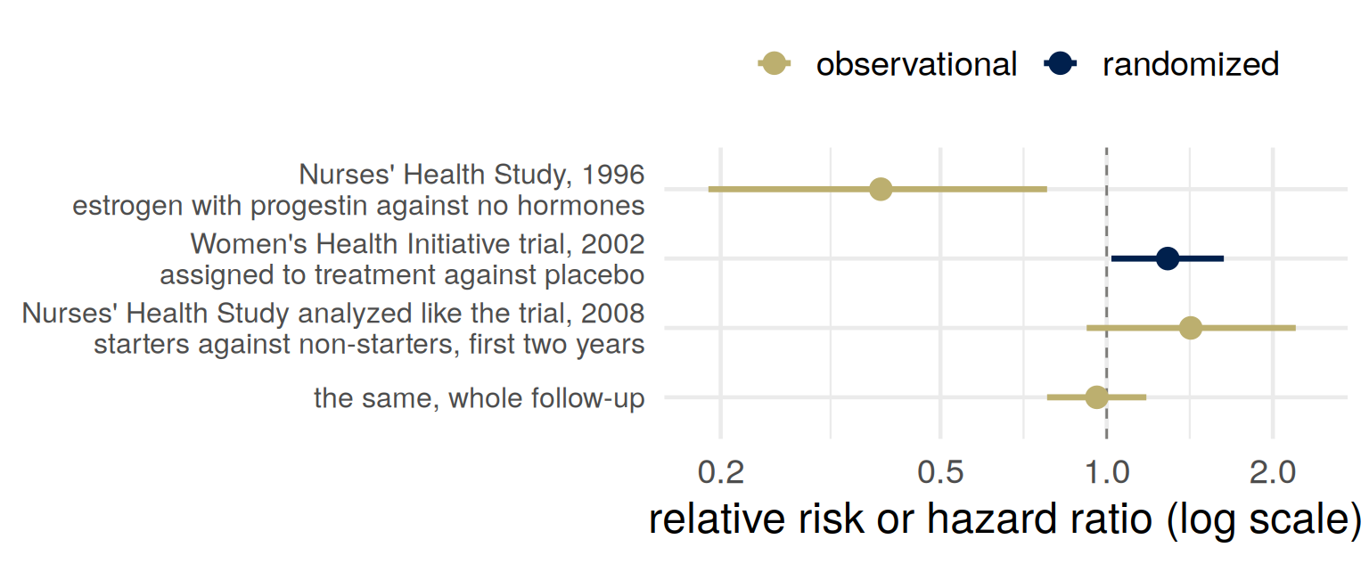
Nurses’ Health Study: 59,337 women, followed for up to 16 years. Women taking estrogen with progestin after the menopause, against women not using hormones:
relative risk of major coronary heart disease 0.39 (95% interval 0.19 to 0.78), adjusted for the confounders the authors measured.
“The addition of progestin does not appear to attenuate the cardioprotective effects of postmenopausal estrogen therapy.”
Grodstein and colleagues (1996), New England Journal of Medicine 335, 453–461.
A trial randomizes women to estrogen with progestin or to a placebo. Write down the ratio you expect for coronary heart disease.
Hormone therapy, 2002 and 2008
Estrogen with progestin “should not be initiated or continued for primary prevention of CHD.”
Writing Group for the Women’s Health Initiative Investigators (2002), JAMA 288, 321–333. Hernán and colleagues (2008), Epidemiology 19, 766–779.
Two explanations
Confounding:
“a suspected beneficial effect of hormone replacement therapy in reducing cardiovascular disease disappeared after identifying socioeconomic status as a confounding variable.”
fairmlbook, chapter 5, citing Humphrey, Chan and Sox (2002): in studies adjusted for socioeconomic status and the major coronary risk factors, relative risk 1.07 (credible interval 0.79 to 1.48).
The comparison: starters against non-starters, followed from the same point, gave estimates “similar to those from the Women’s Health Initiative.”
Hernán and colleagues (2008).
Which comparison gets reported? Women who took hormones against women who did not, or starters against non-starters.
Structural causal models
“a sequence of assignments for generating a joint distribution starting from independent noise variables.”
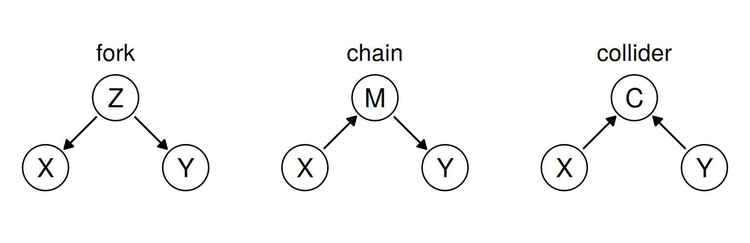
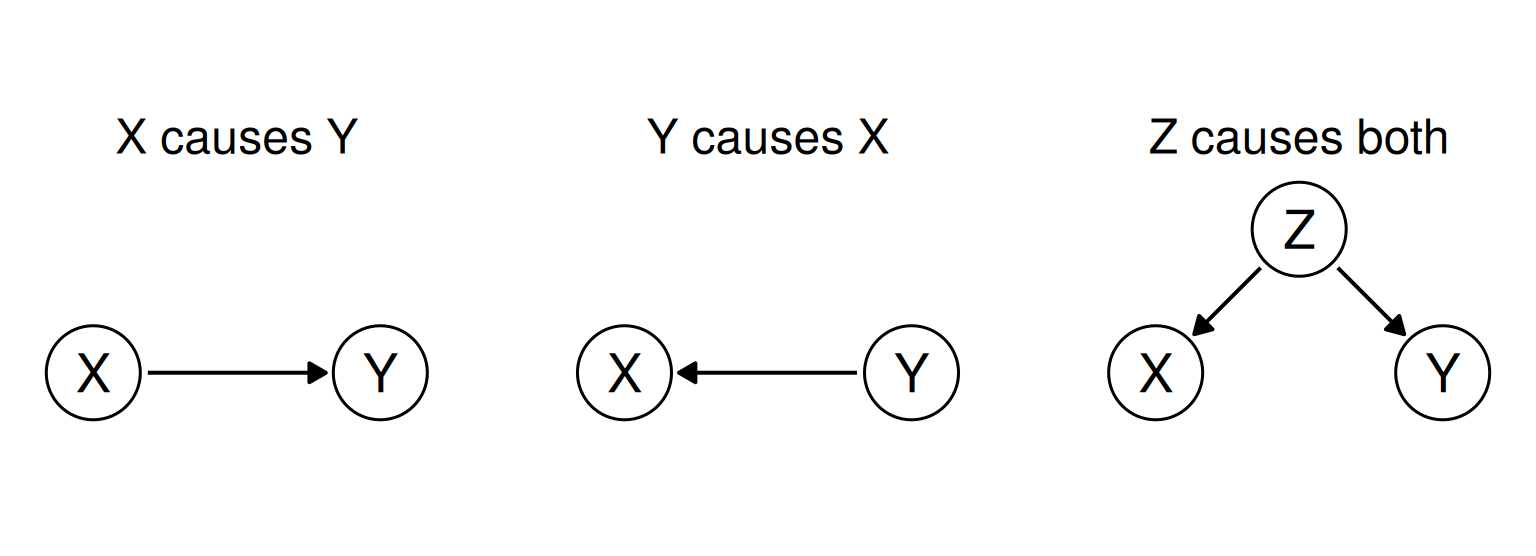
\(Z\) a common cause, \(M\) a mediator, \(C\) a common effect.
fairmlbook, chapter 5, “Causal models” and “Causal graphs.”
Exercise, weight and heart disease
\(U_1 \sim \mathrm{Ber}(1/2)\), \(\;U_2, U_3 \sim \mathrm{Ber}(1/3)\), independent; \(\mathrm{Ber}(q)\) is 1 with probability \(q\).
- \(X := U_1\) (exercise)
- \(W :=\) if \(X = 1\) then \(0\) else \(U_2\) (overweight)
- \(H :=\) if \(X = 1\) then \(0\) else \(U_3\) (heart disease)
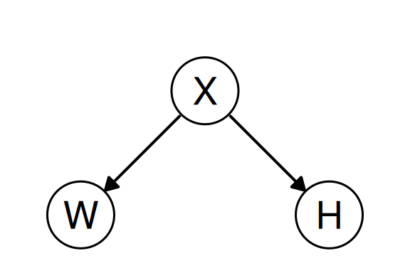
Apart from the noise, an arrow into a variable comes from each variable its line uses: \(W\) and \(H\) are both computed from \(X\).
Compute \(P(H = 1)\) and \(P(H = 1 \mid W = 1)\).
fairmlbook, chapter 5, “A first example.”
Conditioning and intervening
\(P(H = 1) = \tfrac12 \cdot \tfrac13 = \tfrac16\), \(\qquad P(H = 1 \mid W = 1) = \tfrac13\).
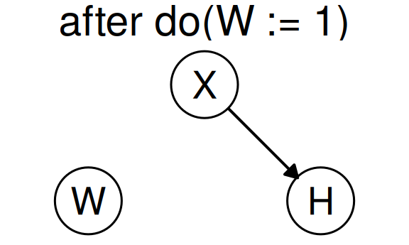
\(do(W := 1)\): replace line 2 by \(W := 1\). In the graph, the arrow into \(W\) is deleted.
\(P(H = 1 \mid do(W := 1)) = \tfrac16\).
“The substitution \(W := 1\) does not correspond to a conditioning on \(W = 1\). One is an action, albeit inconsequential in this case.”
\(X\) and \(Y\) are confounded when \(P(Y = y \mid do(X := x)) \ne P(Y = y \mid X = x)\).
fairmlbook, chapter 5, “A first example” and “Confounding.”
The average treatment effect
\[
\text{ATE} = E[Y \mid do(X := 1)] - E[Y \mid do(X := 0)]
\]
Each term deletes the arrows into \(X\) and sets \(X\) to the same value for everyone.
“Causal effects are population quantities. They refer to effects averaged over the whole population. Often the effect of treatment varies greatly from one individual or group of individuals to another.”
The observed difference \(E[Y \mid X = 1] - E[Y \mid X = 0]\) compares the people who happened to be treated with the people who were not.
fairmlbook, chapter 5, “Causal effects.”
Adding up over people
Suppose \(Y\) measures how well off a person is, on a scale that adds up across people, and nobody’s outcome depends on anyone else’s treatment. Then treating all \(n\) people rather than none changes the expected total of \(Y\) by \(n \times \text{ATE}\): the utilitarian’s comparison of the two actions.
A gain to one person offsets a loss to another. A positive ATE is consistent with some people being made worse off.
Justice, in the Belmont Report, concerns who receives the benefits of research and who bears its burdens. For a policy, what would you need to know besides the ATE?
Wikipedia, Belmont Report.
Prediction and intervention
“If we expect a model to also tell us what happens when we intervene on variables, then […] models with equal predictive accuracy are no longer equivalent. We become responsible to choose one of them.”
Figure 1 of Loftus (2024), “Position: The Causal Revolution Needs Scientific Pragmatism,” ICML.
Draw the graph
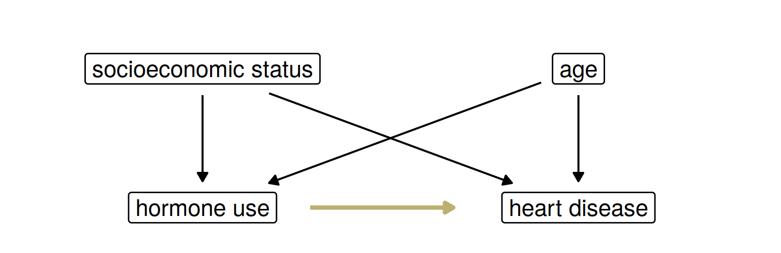
Use hormone use, heart disease, socioeconomic status and age. Draw the graph the 1996 conclusion needs, then add arrows that would make women taking hormones look healthier even if the hormones did nothing.
Hormone therapy: one graph
The gold arrow is the claim that the hormones protect the heart. The four black arrows can produce a difference between users and non-users without it.
Part 3: Confounding and adjustment
A job-search course
A job center refers some of the 1,000 people registered with it to a job-search course. Everyone referred attends, and nobody else does. Six months later:
| 1,000 people |
500, of whom 320 in work (64%) |
500, of whom 180 in work (36%) |
How much does the course raise the chance of being in work? Write down a number, or what else you would need to know.
The rows
| worked last year (\(Z = 1\)), 500 |
400, of whom 280 in work (70%) |
100, of whom 60 (60%) |
| did not (\(Z = 0\)), 500 |
100, of whom 40 in work (40%) |
400, of whom 120 (30%) |
| total, 1,000 |
500, of whom 320 in work (64%) |
500, of whom 180 (36%) |
\(Z\) = worked last year, \(X\) = attended the course, \(Y\) = in work six months later.
The observed comparison
\(Z\) worked last year, \(X\) attended, \(Y\) in work. Each row is weighted by its share of attenders, or of non-attenders:
\[
\begin{aligned}
P(Y = 1 \mid X = 1) &= \frac{0.7 \times 400 + 0.4 \times 100}{500} = 0.64 \\
P(Y = 1 \mid X = 0) &= \frac{0.6 \times 100 + 0.3 \times 400}{500} = 0.36
\end{aligned}
\]
Attenders come mostly from the \(Z = 1\) row, where more people find work whether or not they attend.
Referral at random
Same people, same rows. The center now refers half of each row, chosen at random; everyone referred attends, and nobody else does.
Compute the share in work you would expect among those who attended, and among those who did not. Compare the difference with the average treatment effect.
Randomization
Half of each row attends, chosen at random. The shares to expect:
\[
\begin{aligned}
P(Y = 1 \mid X = 1) &= 0.5 \times 0.7 + 0.5 \times 0.4 = 0.55 \\
P(Y = 1 \mid X = 0) &= 0.5 \times 0.6 + 0.5 \times 0.3 = 0.45
\end{aligned}
\]
The observed difference is the effect, apart from the chance variation of one draw.
“The goal of a randomized controlled trial is to break natural inclination.”
fairmlbook, chapter 5, “Randomization.”
The backdoor criterion
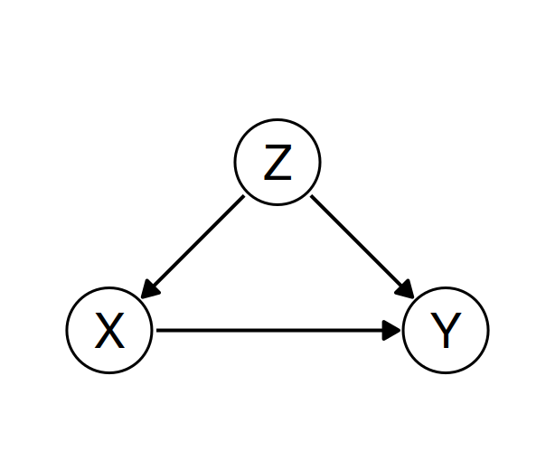
A backdoor path from \(X\) to \(Y\) starts with an arrow into \(X\): here, \(X \leftarrow Z \to Y\).
\(Z\) satisfies the backdoor criterion if
- no variable in \(Z\) is a descendant of \(X\), and
- \(Z\) blocks every backdoor path from \(X\) to \(Y\).
A path through a fork or a chain is blocked by conditioning on the variable in the middle.
Controlling for a mediator “will eliminate some of the causal influence of \(X\) on \(Y\).”
The criterion: Pearl (2009), Causality, as cited in fairmlbook, chapter 5. The quotation: fairmlbook, chapter 5, “Confounding.”
Unobserved confounding
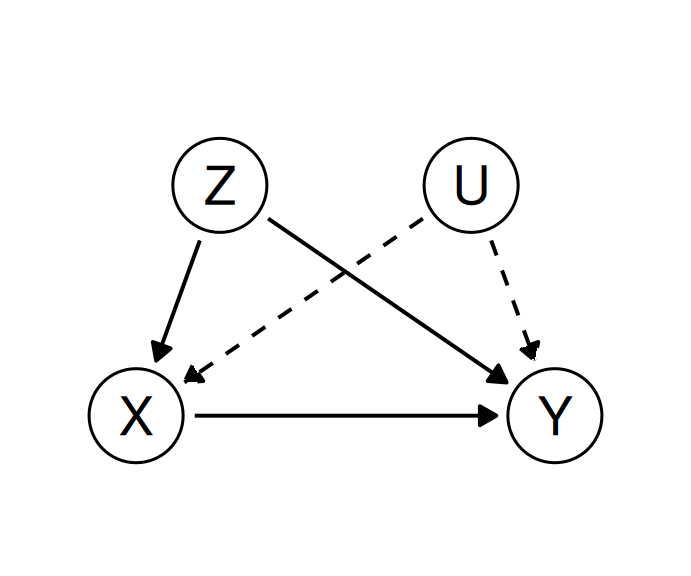
\(U\): something unmeasured, such as motivation, that pushes people onto the course and into work.
Under the graph without \(U\), adjusting for \(Z\) gives the effect. Under this one, the back door through \(U\) stays open, and the 10 points probably overstates the effect.
The data on \(X\), \(Y\) and \(Z\) fit both graphs.
Part 4: Reinforcement learning
Reinforcement learning
Notation: in this part, the letters of reinforcement learning: \(S\) state, \(A\) action, \(R\) reward, \(\pi\) policy, \(U\) utility.
An agent observes a state \(S\), takes an action \(A = \pi(S)\) and receives a reward \(R\). The policy \(\pi\) is a rule for acting. Learning means changing \(\pi\) to make \(E_\pi[R]\) large, the expected reward when the agent acts by \(\pi\).
The good we care about is \(U\). A consequentialist would choose the policy with the largest \(E_\pi[U]\); the agent is given \(R\) instead.
Whether \(E_\pi[U]\) is a causal quantity depends on further assumptions. Causal reinforcement learning, a subfield, brings causal models into reinforcement learning.
A cleaning robot
Notation: reinforcement learning (\(S\), \(A\), \(R\), \(\pi\), \(U\)).
\(S\): what the robot’s camera shows. \(A\): where to move, and whether to clean. \(R\): 1 when no mess is in view. \(U\): a clean room.
Rewarded for not seeing any mess, the robot can earn full reward by closing its eyes, or by covering the mess with something it cannot see through.
Amodei, Olah, Steinhardt, Christiano, Schulman and Mané (2016), “Concrete Problems in AI Safety,” sections 2 and 4.
A job center as an agent
Notation: reinforcement learning (\(S\), \(A\), \(R\), \(\pi\), \(U\)).
A variant of the lecture’s job center: it has 100 places on the course, which here helps some people more than others.
| worked last year |
70% |
64% |
| did not |
40% |
14% |
\(S\): a person’s record. \(A\): refer or not. \(R\): the share of those referred who are in work, the center’s performance measure. \(U\): the number in work because of the course.
Whom does a center judged on \(R\) send? Whom would a utilitarian send?
Cream skimming
Notation: reinforcement learning (\(S\), \(A\), \(R\), \(\pi\), \(U\)).
Send 100 who worked last year: \(R\) = 70%, and \(U\) = 6 more people in work. Send 100 who did not: \(R\) = 40%, and \(U\) = 26 more.
Choosing people who would have found work anyway is called cream skimming. US job-training centers funded under the Job Training Partnership Act were judged partly on employment rates. Economists who studied them found that cream skimming changed the programs’ efficiency little, in either direction, and concluded that “opposition to cream skimming must come on equity grounds.”
Heckman, Heinrich and Smith (2002), “The Performance of Performance Standards,” NBER Working Paper 9002, abstract and section VIII. They also found the short-run measures “weakly, and sometimes perversely, related to long run impacts.”
Utilitarianism with a reward
Notation: reinforcement learning (\(S\), \(A\), \(R\), \(\pi\), \(U\)).
An agent judges a policy only by the reward it expects. That is consequentialism, with the good defined by whoever chose \(R\).
| defining utility |
someone chooses \(R\), and \(R\) is not \(U\) |
| trading off between people |
reward is added up over the people served |
| judging acts or rules |
the policy is a rule: it treats alike everyone in the same state |
| predicting consequences |
a model of what the actions do, which is a causal model |
Lenses this week
- What are we optimizing or predicting? The center’s placement rate, or the jobs the course creates.
- Which comparison gets reported? Attenders against non-attenders, overall or within rows. Women who took hormones against women who did not, or starters against non-starters. The average effect, or the effects within groups defined before treatment.
- You have to choose, so choose, and defend it. The adjustment set follows from a graph you drew. The backdoor criterion says which sets are valid given the graph; it does not draw the graph. “Pretending it was forced is its own failure.”
…and why?
Does consequentialism become more or less defensible once you have to write the causal model down?
For next time: bring one score or algorithm used to make decisions about people, with what it measures and what it stands in for.