Causal models

Summary

Causal models are useful for understanding different kinds of statistical relationships between two or more variables.

References

Assigned reading

• FairML Book Chapter 5 on Causality, at least to the section on Counterfactuals (about halfway through).

Additional references

• FairML Book the rest of Chapter 5.
• Causal Inference: The Mixtape Sections 1.1, 1.2, and 3.1 up to 3.1.3 (stop before 3.1.4)

Notes

Simulating data based on DAGs

Note: we can make nice graphs using the ggdag package to plot graphs.

Graph: \(X \rightarrow Y\)

Original world

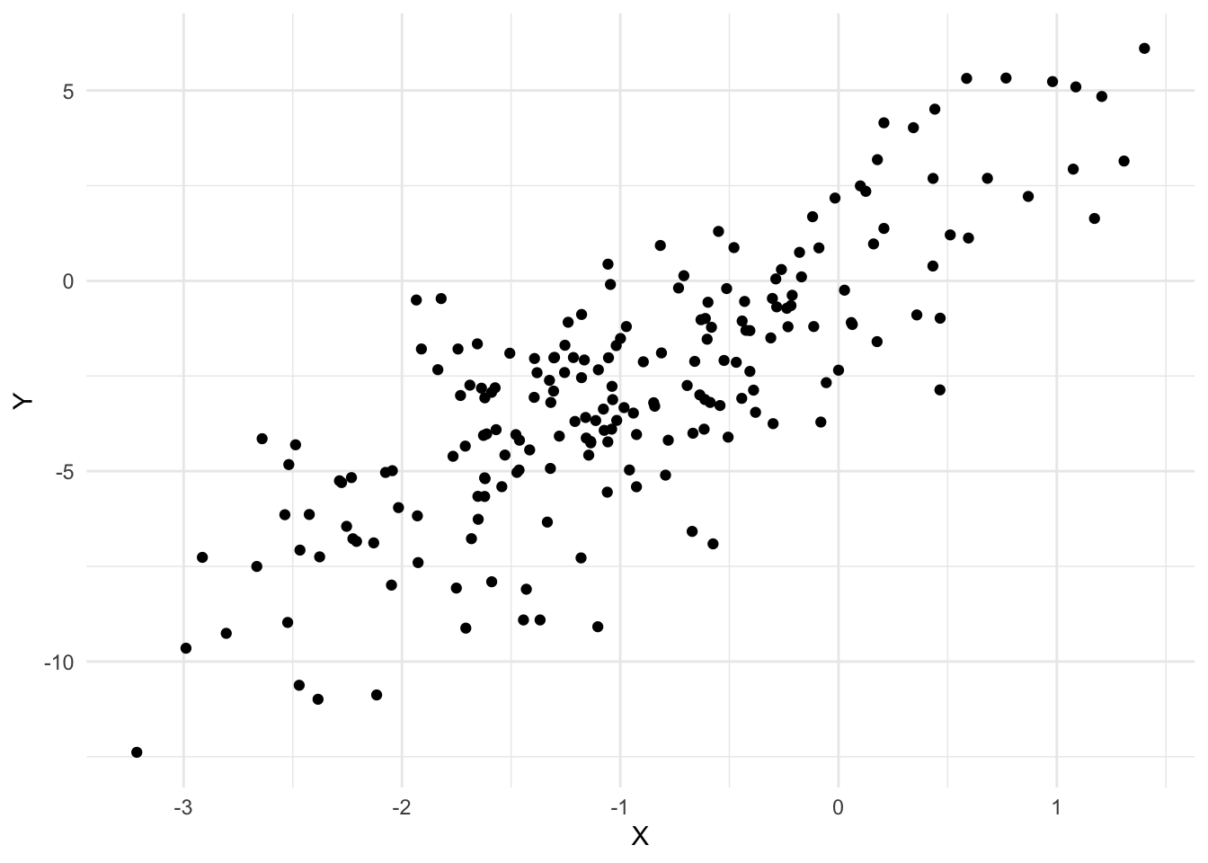
library(tidyverse)
theme_set(theme_minimal())
set.seed(1)
n <- 200
# Step 1: Generate variables with no parents
f_X <- function(noise) noise - 1
noise_X <- rnorm(n)
X <- f_X(noise_X)
# Step k+1: Generate variables that had their
# set of parents finish generating at step k
f_Y <- function(x, noise) 3 * x + 2 * noise
noise_Y <- rnorm(n)
Y <- f_Y(X, noise_Y)
qplot(X, Y)

Sample average of Y:

mean(Y)

[1] -2.812106

World after intervention

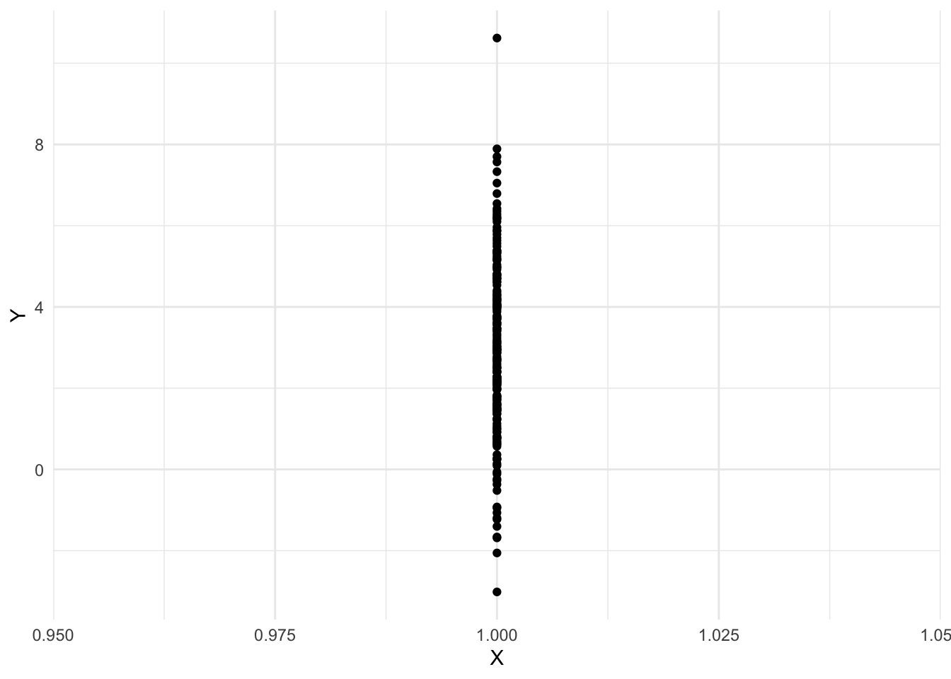
We start by copying and pasting the original code, then we modify the program to change some variable. In this case we do an “atomic” intervention setting all \(X\) values to 1.

Since the code is written in a way that any variables depending on \(X\) (in this graph \(Y\) does) are generated after \(X\), this intervention on \(X\) may change their distributions as well.

# Step 1: Generate variables with no parents
X <- 1
# Step k+1: Generate variables that had their
# set of parents finish generating at step k
f_Y <- function(x, noise) 3 * x + 2 * noise
noise_Y <- rnorm(n)
Y <- f_Y(X, noise_Y)
qplot(X, Y)

Sample average of Y:

mean(Y)

[1] 2.916346

Explanation

With this simple data generating process we can see that \(X \sim N(-1, 1)\) and \((Y | X = x) \sim N(3x, 4)\). By linearity, \(E[Y] = 3E[X] = -3\) in the original world. But after the intervention \(\text{do}(X := 1)\), we have \(E[Y] = 3 E[1] = 3 \cdot 1 = 3\).

Graph: \(X \leftarrow U \rightarrow Y\)

Original world

n <- 10000 # reduce sampling variability
# Step 1: Generate variables with no parents
U <- rnorm(n)
# Step k+1: Generate variables that had their
# set of parents finish generating at step k
f_X <- function(u, noise) 2 * u + 3 + noise
noise_X <- rnorm(n)
X <- f_X(U, noise_X)
f_Y <- function(u, noise) u^2 + noise^2
noise_Y <- rnorm(n)
Y <- f_Y(U, noise_Y)

Sample average of Y:

mean(Y)

[1] 2.030961

World after intervention

An “atomic” intervention setting all X values to 1.

# Step 1: Generate variables with no parents
U <- rnorm(n)
# Step k+1: Generate variables that had their
# set of parents finish generating at step k
X <- 1
f_Y <- function(u, noise) u^2 + noise^2
noise_Y <- rnorm(n)
Y <- f_Y(U, noise_Y)

Sample average of Y:

mean(Y)

[1] 2.032377

Explanation

In this case the mean of \(Y\) did not change because the variable we intervened on, \(X\), is not a cause of \(Y\).