generate_data <- function(beta0 = 0,
                          betaX = 0,
                          betaA = 0,
                          betaXA = 0,
                          n = 200,
                          proportion = 1/2) {
  X <- rnorm(n)
  A <- rbinom(n, 1, proportion)
  Y <- beta0 + betaX * X + betaA * A + betaXA * X * A + rnorm(n, sd = 1)
  data.frame(Y = Y, X = X, A = factor(A))
}Ethics4DS: Coursework 1
Reproducibility
Change parameters of the simulation as necessary (or as desired, to make it unique)
Here is a visualisation to help understand the data
one_sample <- generate_data(beta0 = 2, betaX = -1, betaA = 2, betaXA = 1.5)
one_sample |>
  ggplot(aes(X, Y, color = A)) +
  geom_point() +
  geom_smooth(method = "lm", se = FALSE)
`geom_smooth()` using formula = 'y ~ x'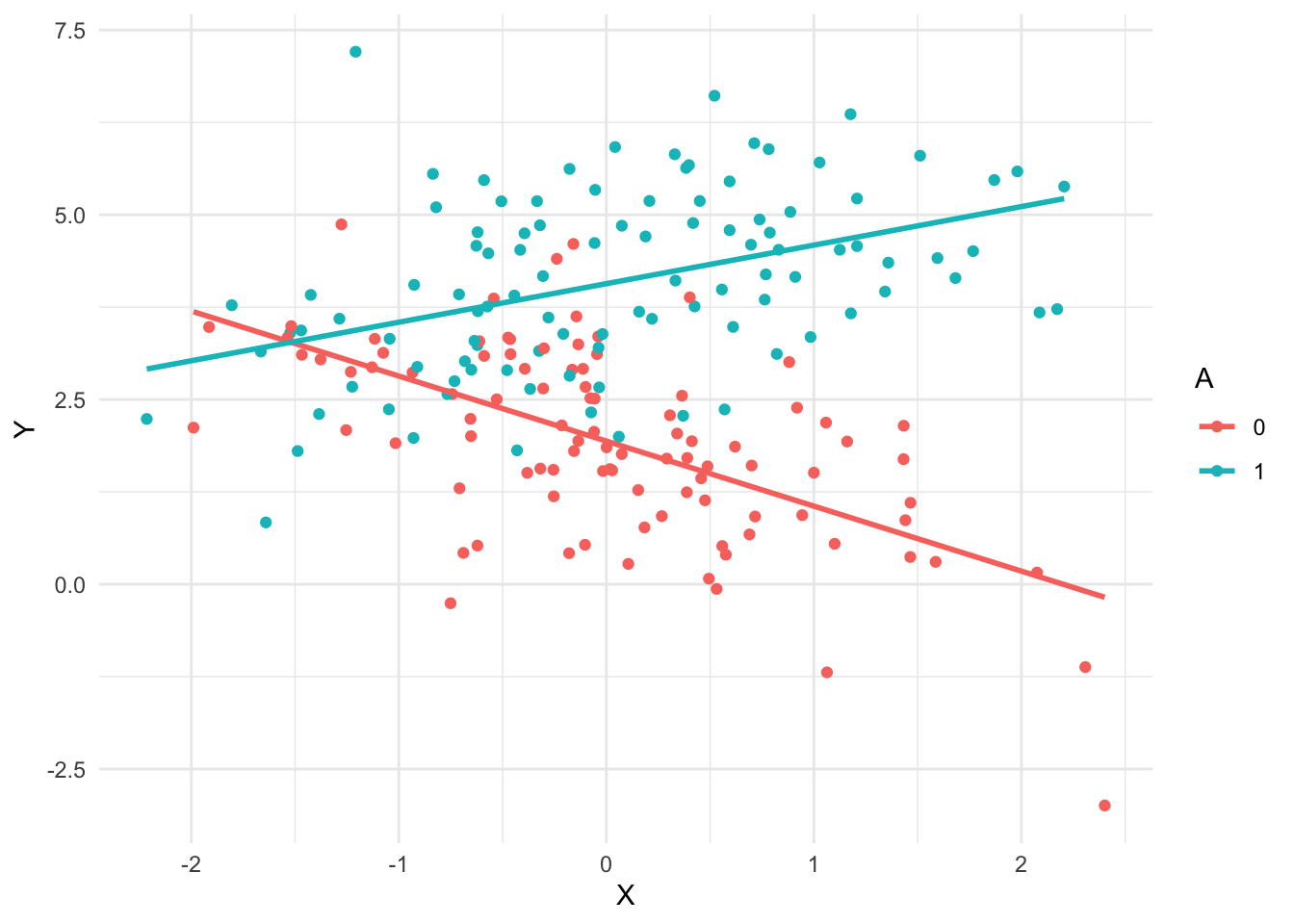
one_fit <- lm(Y ~ X + A + X * A, one_sample)
summary(one_fit)
Call:
lm(formula = Y ~ X + A + X * A, data = one_sample)

Residuals:
    Min      1Q  Median      3Q     Max
-2.8553 -0.6802 -0.0024  0.6824  3.7687

Coefficients:
            Estimate Std. Error t value Pr(>|t|)
(Intercept)   1.9373     0.1103  17.560  < 2e-16 ***
X            -0.8801     0.1258  -6.994  4.1e-11 ***
A1            2.1303     0.1538  13.851  < 2e-16 ***
X:A1          1.4017     0.1672   8.381  1.0e-14 ***
---
Signif. codes:  0 '***' 0.001 '**' 0.01 '*' 0.05 '.' 0.1 ' ' 1

Residual standard error: 1.086 on 196 degrees of freedom
Multiple R-squared:  0.5808,    Adjusted R-squared:  0.5744
F-statistic: 90.53 on 3 and 196 DF, p-value: < 2.2e-16summary(one_fit)$coefficients[,4] (Intercept) X A1 X:A1
4.291280e-42 4.101667e-11 7.199416e-31 1.004225e-14 # p-values for all the non-intercept variables
summary(one_fit)$coefficients[-1,4] X A1 X:A1
4.101667e-11 7.199416e-31 1.004225e-14 # p-value for second coeff
summary(one_fit)$coefficients[2,4][1] 4.101667e-11# Every time this function is called, it:
# (1) generates new data
# (2) fits a model using the formula Y ~ X + A + X * A
# (3) returns the p-value for the second coefficient
one_experiment <- function(beta0 = 0, betaX = 0, betaA = 0,
betaXA = 0, n = 200, proportion = 1/2) {
one_sample <- generate_data(beta0, betaX, betaA, betaXA, n, proportion)
one_fit <- lm(Y ~ X + A + X * A, one_sample)
p_values <- summary(one_fit)$coefficients[2,4]
return(p_values)
}one_experiment()[1] 0.8266538one_experiment(betaX = .3)[1] 0.1502811n_experiments <- 5
replicate(n_experiments, one_experiment())[1] 0.9677839 0.5647648 0.1151294 0.2137763 0.7461851rejection_level <- 0.05
n_experiments <- 500
# proportion of experiments where p-value
# is below rejection level
mean(replicate(n_experiments, one_experiment()) < rejection_level)[1] 0.032Consider: What should this be? Is the above result acceptable or concerning?
mean(replicate(n_experiments, one_experiment(betaX = .2)) < rejection_level)[1] 0.474A larger proportion of experiments had significant p-values this time. Is that what we expect?
How would this rejection rate depend on each of the parameters input to the one_experiment() function (e.g. betaX, betaA, n, etc)?
When do we want the rejection rate to be high, and when do we want it to be low?
Note: it may be helpful to review basic conditional control flow in R from sources like one of the following
Instructions: after completing the rest of this notebook, delete this comment and all of the demonstration code above. You should only keep the code necessary for your answers below to work.
Preregistration vs p-hacking
p-hacking
- Modify the example code to create a function that simulates p-hacking
- Show the effect of p-hacking on statistical error rates using any appropriate statistics or visualisations that you prefer
- Explain, in your own words, what problems could result from p-hacking
one_phacked_experiment <- function(beta0 = 0, betaX = 0, betaA = 0,
                           betaXA = 0, n = 200, proportion = 1/2) {
  one_sample <- generate_data(beta0, betaX, betaA, betaXA, n, proportion)
  one_fit <- lm(Y ~ X + A + X * A, one_sample)
  min_pvalue <- min(summary(one_fit)$coefficients[-1,4])
  another_fit <- lm(Y ~ X, one_sample)
  another_pvalue <- summary(another_fit)$coefficients[2,4]
  p_values <- min(min_pvalue, another_pvalue)
  return(p_values)
}
rejection_level <- 0.05
n_experiments <- 500
# proportion of experiments where p-value
# is below rejection level
all_experiments_pvalues <- replicate(n_experiments, one_phacked_experiment())
mean(all_experiments_pvalues < rejection_level)[1] 0.172hist(all_experiments_pvalues)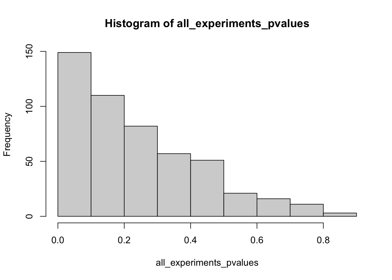
Preregistration
- Create another version of the function to simulate the constraints of preregistration
- Compare the error rates with preregistration to those without, and explain whether this could help with any problems you identified above and, if so, how
one_preregistered_experiment <- function(beta0 = 0, betaX = 0, betaA = 0,
                           betaXA = 0, n = 200, proportion = 1/2) {
  one_sample <- generate_data(beta0, betaX, betaA, betaXA, n, proportion)
  one_fit <- lm(Y ~ X + A + X * A, one_sample)
  several_pvalues <- summary(one_fit)$coefficients[-1,4]
  another_fit <- lm(Y ~ X, one_sample)
  another_pvalue <- summary(another_fit)$coefficients[2,4]
  p_values <- c(several_pvalues, another_pvalue)
  return(p_values)
}
rejection_level <- 0.05
n_experiments <- 500
# proportion of experiments where p-value
# is below rejection level
all_experiments_pvalues <- replicate(n_experiments, one_preregistered_experiment())
mean(all_experiments_pvalues < rejection_level)[1] 0.054hist(all_experiments_pvalues)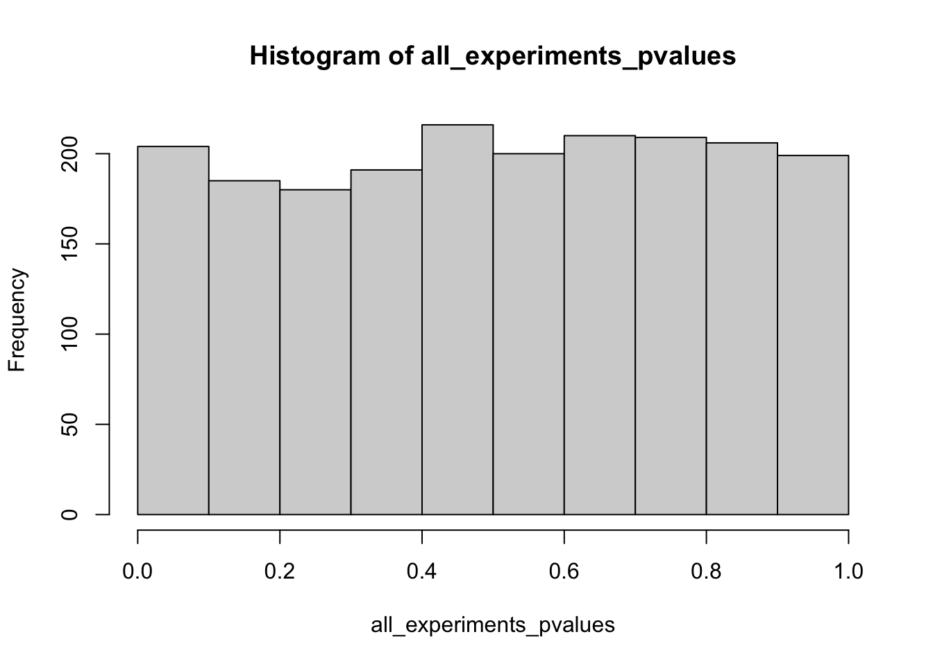
Reproducibility and causality
Reproducible and causal
- Create another simulation, modifying the data generating code to be consistent with a specific causal model structure, and choosing the structure to satisfy the following the following requirements
- Show that there is a reproducible effect, i.e. one that can be found fairly consistently (e.g. in more than five percent of experiments) without using p-hacking
- Show, by simulating an intervention, that the above effect is causal
# no changes necessary from original experiment
# if true betaX is nonzero then rejections are not false discoveries
# rejection rate:
mean(replicate(n_experiments, one_experiment(betaX = .2)) < rejection_level)
[1] 0.47Why is this effect causal?
Assuming the code that generates the data accurately represents a causal model, we see the function generating Y depends on X. So if X is intervened on, then Y will also change. Here’s a simple example showing the effect:
# Using betaX = .2, all other coeffs = 0
N <- 1000 # reduce sampling variation

# Before intervention
X <- rnorm(N)
A <- rbinom(N, 1, 1/2)
Y <- 0.2 * X + rnorm(N, sd = 1)

# After intervention
X_new <- 2
A_new <- rbinom(N, 1, 1/2)
Y_new <- 0.2 * X_new + rnorm(N, sd = 1)

mean(Y_new) - mean(Y)
[1] 0.4127188This shows that an intervention setting every value of X to 2 (for example) results in a different average value of Y
Conclusion: there is a true causal effect, and regression experiments find a statistically significant coefficient for X (with a rejection rate that is higher than 0.05)
Reproducible but not causal
- Repeat the above section, but in this case choose the causal model generating your data so that the reproducible effect is not causal, i.e. an intervention on that variable does not change the outcome variable
generate_common_cause_data <- function(n = 100,
                                    sdx = .2,
                                    sdy = .2,
                                    intervention = NULL) {

  # Original world
  # Y <- U -> X
  U <- rnorm(n) # unobserved
  f_X <- function(U) U + 1
  f_Y <- function(U) (1/5) * (1 + U)^2

  X <- f_X(U) + rnorm(n, sd = sdx)
  Y <- f_Y(U) + rnorm(n, sd = sdy)

  # Optional: intervene on X
  if (!is.null(intervention)) {
    # Intervened world
    # Y <- U, X <- intervention
    # U is generated before X
    U <- rnorm(n)
    # X is set to a specific value
    X <- intervention
    # Y is generated after X, but keeps its original
    # distribution because f_Y does not use X
    Y <- f_Y(U) + rnorm(n, sd = sdy)
  }

  data.frame(Y = Y, X = X)
}
Original data
one_common_cause_dataset <- generate_common_cause_data(n = 400)
ggplot(one_common_cause_dataset, aes(X, Y)) +
  geom_point(alpha = .5) +
  geom_smooth(method = "lm", se = FALSE)
`geom_smooth()` using formula = 'y ~ x'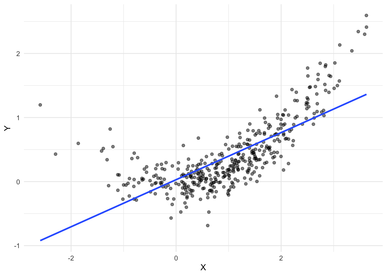
Data with an intervention setting X to 1
intervened_common_cause_dataset <-
  generate_common_cause_data(n = 400, intervention = 1)
ggplot(intervened_common_cause_dataset, aes(X, Y)) +
  geom_point(alpha = .5) +
  geom_smooth(method = "lm", se = FALSE)
`geom_smooth()` using formula = 'y ~ x'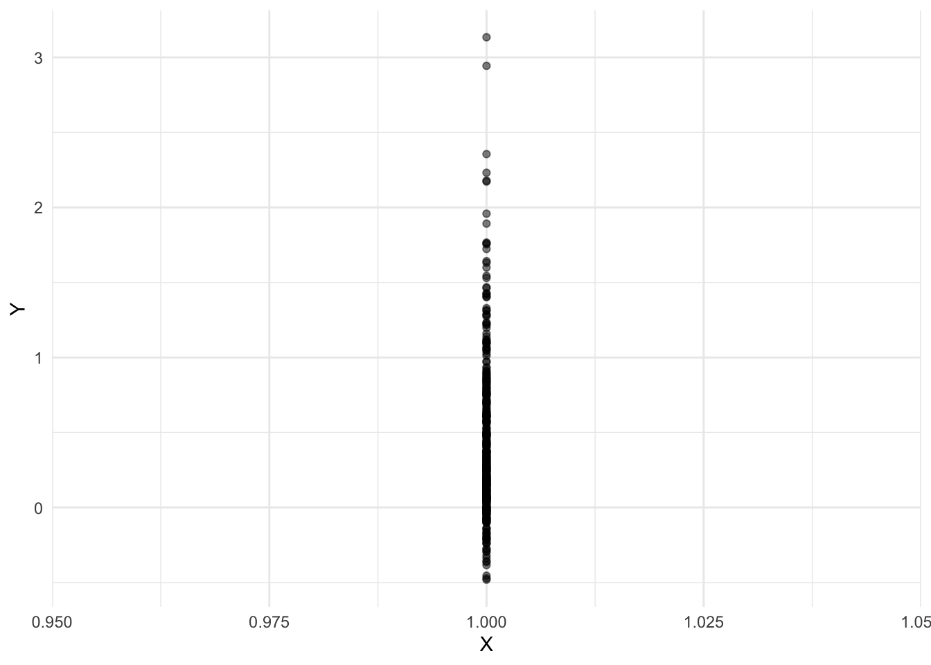
Averages of Y before and after intervention
mean(one_common_cause_dataset$Y)[1] 0.3960258mean(intervened_common_cause_dataset$Y)[1] 0.4258304Simulate one experiment
# Every time this function is called, it:
# (1) generates new "common cause" data
# (2) fits a model using the formula Y ~ X
# (3) generates "common cause" data with intervention on X
# (4) computes mean of Y before and after intervention
# returns: X coefficient and p-value from (2), interventional effect (4)
one_common_cause_experiment <- function(n = 100,
                                      sdx = .2,
                                      sdy = .2,
                                      intervention = 1) {
  # without intervention
  one_sample <- generate_common_cause_data(n, sdx, sdy)
  one_fit <- lm(Y ~ X, one_sample)
  beta_hat <- summary(one_fit)$coefficients[2,1]
  p_value <- summary(one_fit)$coefficients[2,4]

  # with intervention
  intervened_sample <- generate_common_cause_data(n, sdx, sdy, intervention)
  avg_Y_diff <- mean(intervened_sample$Y) - mean(one_sample$Y)
  return(list(beta_hat = beta_hat,
              p_value = p_value,
              intervention_effect = avg_Y_diff))
}
Simulate multiple experiments and transform the results to make them easy to plot
multiple_common_cause_experiments <- function(n_experiments = 200,
                                              n = 100,
                                              sdx = .2,
                                              sdy = .2,
                                              intervention = 1) {
  experiment_summary_list <- replicate(
    n_experiments,
    one_common_cause_experiment(n, sdx, sdy, intervention))
  experiment_summaries <- apply(t(experiment_summary_list), 2, unlist)
  return(data.frame(experiment_summaries))
}
experiment_summaries <- multiple_common_cause_experiments()Distribution of estimated coefficients for X
ggplot(experiment_summaries, aes(beta_hat)) + geom_histogram(bins = 20)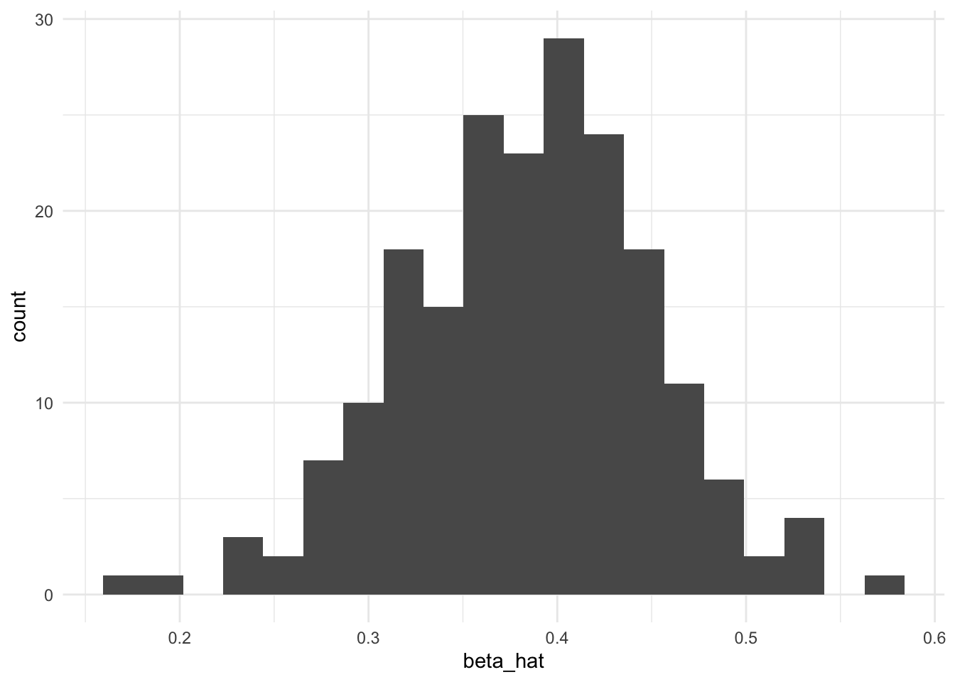
Rejection rate using p-values for X
rejection_level <- 0.05
# proportion of experiments where p-value
# is below rejection level
mean(experiment_summaries$p_value < rejection_level)
[1] 1Distribution of mean difference in Y when intervening on X
ggplot(experiment_summaries, aes(intervention_effect)) +
  geom_histogram(bins = 20)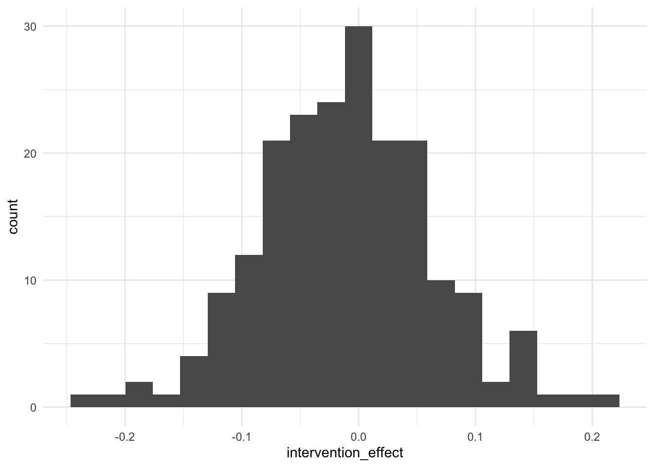
Average interventional effect across multiple experiments (meta-analysis)
mean(experiment_summaries$intervention_effect)[1] -0.01083109Conclusion: experiments consistently find a statistically significant coefficient for X (without using p-hacking to achieve significance), and yet there is no causal effect of X on Y (their significant association is due to having a common cause U, which in our simulation is unobserved by the experimenter)